My name is Vince Knight and I'm a lecturer in Operational Research at Cardiff University with interests in game theory and queueing theory. I'll be using this blog to post about various things mainly including math and software...
www.vincent-knight.com
The other great reason why this is awesome is that it just got really easy to use and install Sage.
Here's a short video demonstrating everything I've done below:
If you're familiar with git then you know this but if you're not then you can simply open up a terminal on anything *nix (linux/Mac OS) and type the following:
$ cd ~ $ git clone git://github.com/sagemath/sage.git This basically goes to the git repository on github and clones it to a folder called sage in your home directory (if you don't have git installed you'll have to do that first). Once you've done that you need to 'make' sage: $ cd ~/sage $ make This will take a little while (it goes and gets most of what you need so it's hard to say how long as it depends on your machine) but after that you'll have Sage on your machine. If you're still in the ~/sage directory you can simply type ./sage to start sage. You'll want to add sage to your path so that you can use it from any directory. In this video I did this by using a bit of a trick but here's I'll do something simpler: create a symbolic link to the sage file in ~/sage directory and place that symbolic link in your path (in /usr/bin/local). To do that type this: $ ln -s ~/sage/sage /usr/local/bin/sage Now you can type sage anywhere and you'll get sage up and running. What's really great about all this is that if and when updates/development happens you can just git pull to get all up to date changes. Based on the +Sage Mathematical Software System post on G+: here: it looks like you can already play around with the develop branch... Awesome.
Of course if you want the easiest way to use Sage then simply grab an account on +The Sagemath Cloud. I gave a talk last week at the Cardiff Django/Python user group about it and +William Stein was kind enough to drop in and take some questions: http://www.youtube.com/watch?v=OYVLoTL4xt8 (sound quality isn't always great because I move around a fair bit...)
This is one of those: 'writing this post to make sure I remember how I've done this'.
+William Stein posted about bup which he is using to backup +The Sagemath Cloud (if you haven't seen that before make sure you go check it out, here's a video in which I describe it: http://goo.gl/5DtYQq).
bup is a piece of backup software based on git. Here's a talk by +Zoran Zaric explaining it:
Anyway, here's how I setup bup to work like apple's time machine.
Once bup is installed (super easy following readme instruction on Mac OSX and ubuntu). I run:
$ bup -d pathtochosenharddrive init
By default bup uses the ~/.bup directory for everthing. Using the -d flag tells bup to run whatever command (in the above instance: init) in a chosen hard drive. If you're happy to backup to your ~ then ignore all instances of -d pathtochosenharddrive in the following. (Note you can also change $BUP_DIR to take care of this, and you'll also need to know the path to your given hard drive). This initialises a git repository (you only need to do this once really). I put the following in a script (backup.sh): bup -d pathtochosenharddrive index -ux /directorytobackup bup -d pathtochosenharddrive save -n backupname /directorytobackup The first line indexes the files (the -ux flags are something to do with recursively going through the files: type man bup index to read more). The second line checks the index and then saves all files as required (giving them a name). To setup this backup script to run every hour I write the following to a txt file (crontab.txt): 0 */1 * * * globalpathtobackupscript/backup.sh
To add this to the cron jobs:
$ crontab crontab.txt If you type: $ crontab -l You should see the the contents of the crontab.txt file now added to the scheduled jobs. The first 0 implies that it'll run at the 0th minute, the */1 means every one hour (so you can easily change this), the other * mean 'every', day, month and day of the week. The first time you run this it should take a fair while (especially if you're backing up your whole ~) but afterwards it shouldn't take too long at all. To check what bup has done, run: $ bup -d pathtochosenharddrive ls That should return:
backupname/ and/or any other names of backups. If you want to see the actual backup snapshots:
$ bup -d pathtochosenharddrive ls backupname which will return a list of timestamped snapshots. This has been working pretty seamlessly for a week for me now and I'm probably going to set it up on my work Mac instead of timemachine.
A PhD students recently had a hard time placing floats (figures and table environments) where they wanted in their LaTeX document. I also have just finished teaching LaTeX to all our first years here at +Cardiff University so I thought I'd brush up on my own understanding of these things to make sure that I was explaining things correctly.
I stumbled on the following stackoverflow TeX.Stackexchange (thanks to +Torbjørn Taskjelle for pointing out this and other mistakes) answer: http://goo.gl/A9iJnP
Here's a +writeLaTeX document working through some examples showing the various options that allow you to control floats within the default restrictions: https://www.writelatex.com/read/qkjpvqptqrwd (at the moment that's a read only link but I've suggested it as a template to the writeLaTeX team in case it's useful to anyone). EDIT: Here's the link to the template: http://goo.gl/UmLFr3
I think that reading through the code (which explains how I understand these things to work) could prove helpful when trying to explain how the various options work. Once that's done I'd suggest playing with the following options on the rabbit figure:
Last week I read this blog post by +Patrick Honner. In the post +Patrick Honner plots a graph of a function with a removable discontinuity on Desmos and when zooming in enough he got some errors.
I was waiting around to start this (ridiculously fun) Hangout on Air with a bunch of mathematicians hosted by +Amy Robinson of +Science on Google+:
While waiting I rushed to write this blog post claiming that if you did the same thing with +Sage Mathematical Software System you did not get any errors. It was quickly pointed out to me on twitter and in the comments that I just had not zoomed in enough.
I edited the blog post to first of all change the title (it was originally 'When Sage doesn't fail' but now reads 'When Sage also fails') and also to include some code that shows that the exact same error appears.
On G+, +Robert Jacobson (who's the owner of the Mathematics community which you should check out if you haven't already) pointed out that you could surely use Sage's exact number fields to avoid this error.
He put together some code and shared it with me on +The Sagemath Cloud that does exactly this. Here's a slight tweak of the code Robert wrote (hopefully you haven't changed your mind and still don't mind if I blog this Robert!):
f(x) = (x + 2) / (x ^ 2 + 3 * x + 2) # Define the function
discontinuity = -1  # The above function has two discontinuities, this one I don't want to plot
hole = -2  # The hole described by Patrick Honner

def make_list_for_plot(f, use_floats=False, zoom_level=10^7, points=1001):
    count = 0  # Adding this to count how many tries fail
    z = zoom_level
    xmin = hole - 10/z # Setting lower bound for plot
    xmax = min(hole + 10/z, discontinuity - 1/10) # Setting upper bound for plot only up until the second (messy) discontinuity
    x_vals = srange(start=xmin, end=xmax, step=(xmax-xmin)/(points-1), universe=QQ, check=True, include_endpoint=True)

    # If we are using floating point arithmetic, cast all QQ numbers to floating point numbers using the n() function.
    if use_floats:
        x_vals = map(n, x_vals)

    lst = []
    for x in x_vals:
        if x != hole and x != discontinuity:  # Robert originally had a try/except statement here to pick up ANY discontinuities. This is not as good but I thought was a bit fairer...
            y = f(x)
            lst.append((x, y))

    return lst
The code above makes sure we stay away from the discontinuity but also allows us to swap over to floating point arithmetic to see the effect. The following plots the functions using exact arithmetic:
exact_arithmetic = make_list_for_plot(f)

p = list_plot(exact_arithmetic, plotjoined=True)  # Plot f
p += point([hole, -1], color='red', size=30)  # Add a point
show(p)
We see the plot here (with no errors):
To call the plots with floating point arithmetic:
float_arithmetic = make_list_for_plot(f, use_floats=True)

p = list_plot(float_arithmetic, plotjoined=True)  # Plot f
p += point([hole, -1], color='red', size=30)  # Add a point
show(p)
We see that we now get the numerical error:
Just to confirm here is the same two plots with an even higher zoom:
To change the zoom, try out the code in the sage cell linked here: simply change the zoom_level which was set to $10^12$ for the last two plots.
(Going any higher than $10^14$ seems to bring in another error that does not get picked up by my if statement in my function definition: Robert originally had a tryexcept method but I thought that in a way this was a 'fairer' way of doing things. Ultimately though it's very possible and easy to get an error-less plot.)
+Patrick Honner wrote a post titled: 'When Desmos Fails' which you should go read. In it he shows a quirk about Desmos (a free online graphing calculator) that seems to not be able to correctly graph around the removable discontinuity $(-2,-1)$ of the following function:
$$f(x)=\frac{x+2}{x^2+3x+2}$$
People who understand this better than me say it might have something to how javascript handles floats...
Anyway I thought I'd see how +Sage Mathematical Software System could handle this. Here's a Sage cell with an interact that allows you to zoom in on the point (click on evaluate and it should run, it doesn't seem to fit too nice embedded in my blog so here's a link to a standalone Sage cell: http://goo.gl/WtezZ4):
It looks like Sage doesn't have the same issues as Desmos does. This is probably not a fair comparison, and needed a bit more work than Desmos (which I can't say I've used a lot) to get running but I thought it was worth taking a look at :)
EDIT: IF you Zoom in more you do get the same behaviour as Desmos! I thought I had zoomed in to the same level as +Patrick Honner did but perhaps I misjudged from his picture :)
Here's the same thing in Sage (when setting $z=10^7$ in the above code):
I spent a couple of minutes googleing and found various command that would plot complex functions:
f = sqrt(x) + 1 / x
complex_plot(sqrt, (-5,5), (-5, 5))
This gives the following plot:
This was however not what my student was asking. They wanted to know how to plot a given set of points in the complex plain (referred to as the Argand plane). A quick google to check if there was anything in Sage pre built for this brought me to this published sheet by +Jason Grout.
I tweaked it slightly so that it was in line with the commands my students have learnt so far and also to include axes legends and put the following in to a function:
def complex_point_plot(pts): """ A function that returns a plot of a list of complex points. Arguments: pts (a list of complex numbers) Outputs: A list plot of the imaginary numbers """ return list_plot([(real(i), imag(i)) for i in pts], axes_labels = ['Re($z$)', 'Im($z$)'], size=30)
This function simply returns a plot as required. Here is a small test with the output:
Here is some code that will plot the unit circle using the $z=e^{i\theta}$ notation for complex numbers (and the Sage srange command):
pts = [e^(I*(theta)) for theta in srange(0, 2*pi, .1)] complex_point_plot(pts)
Here is the output:
I published all this in a worksheet on our server so it's now immediately available to all our students. I'm really enjoying teaching +Sage Mathematical Software System to our students.
A Sage cell with the above code (that you can run in your browser) can be found here: http://goo.gl/jipzxV
EDIT: Since posting this +Punarbasu Purkayastha pointed out on G+ that list_plot can handle complex points right out of the box :) So the above can just be obtained by typing:
pts = [e^(I*(theta)) for theta in srange(0, 2*pi, .1)]
In this post I thought I'd join in and briefly share the kit I carry around in my backpack and the stuff I use on a day to day basis software wise.
Hardware
Here is a picture of the usual contents of my backpack:
In there you see:
- My tablet (a nexus 7). I use this mainly to read papers and books but also for some teaching stuff where I use it to tick student progress on +Google Drive.
- My smartphone (a nexus 4). I'm kind of addicted to my phone. I use it for email, +Google+, Google Keep, and to remember where I have to be and when (if it's not in my calendar I won't be there: the reverse not necessarily being guaranteed either...).
- My 11" macbook air. This I probably care about more than my wife. I'll talk about software below but it's really from a hardware point of view that I love this machine. So portable and just the right size. I've been really tempted by the +DellXPS 13 Developer edition laptop but the screen size (13") puts me off a bit. I love my big monitors for my desktop but for a laptop I think 11" is perfect (the fact that +Linus Torvalds uses it is also kind of cool).
- The dongle to let me connect my macbook to a projector (kind of annoying that you need this but oh well...).
- An actual paper on paper (every now and then I have a paper in my bag as opposed to reading on my tablet: I happened to have one in there today). I've just done a screencast about the particular paper I'm looking at.
- A 250GB hard drive for backups (I'm pretty paranoid about backups).
- My +Moleskine notebook. For the past 3 or 4 years I've only been using this notebooks and make sure I date them so that I've got a tidy record of all my scribblings on my bookshelf in the office. I got this one autographed by Jorge Cham of +PHD Comics:
- My 4 color Bic pen. I used these throughout highschool but 'lost my way' during University. Just started using them again and remember how awesome they are: always work, nice to have the colours and perfect balance for finger spinning (it might be because I spent most of highschool learning how to finger spin with them).
- A usb stick but I very rarely use it (it was in my backpack when I wrote this).
EDIT: After +Rodolfo Carvajal asked on G+ here's a photo of the backpack itself:
I've had it for about 4 years now and it's an Eastpack (I pretty much try to refuse to use anything else as I learnt to love how durable they were during highschool). It's got a nice padded section for my laptop and straps that I can hook my water bottle too but also that I can use to compress the bag when it's empty (the stuff I carry in it does not take much space). It will be a very sad day when (if?) this bag dies as it's by far my favourite backpack ever (pretty much just being compared against other Eastpacks). There are various other tiny bits of kit that I'm missing here (laser pointer, portable battery) but that's because I've left them somewhere and weren't in the backpack when I got the stuff out to take the photo...
2nd EDIT: They still make the backpack! :) http://goo.gl/Vv4STR
It's a really cool result and one that has given rise to a lot more research (including what I mainly enjoy looking at).
I was asked recently be a colleague to give a 15 minute talk about my research to her second year OR class who will have just seen some queueing theory. I decided to talk about Naor's paper and thought that it would be nice if I could give a graphical representation of the customers arriving at the queue (similar to the DES package: +SIMUL8). So I spent some time writing a simulation engine and using the in built +Python Turtle library to get some graphics. A part from some of the optional plotting (matplotlib), this only uses base python libraries. Here's a gif from an early prototype:
Here's a video discussing Naor's result and showing demonstrating everything with my simulation model:
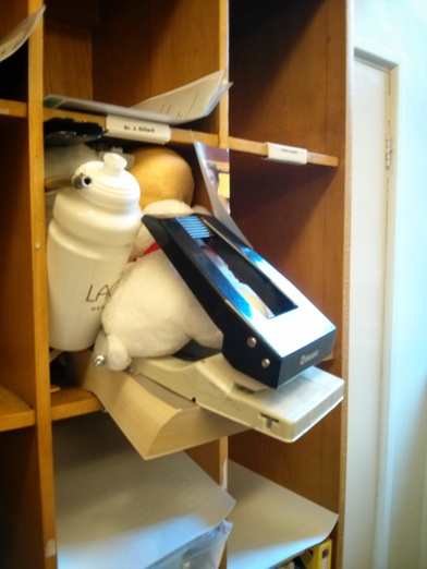
For a while now there's been a 'game' going on with our pigeon holes where people would put random objects in other people's pigeon holes (like the water bottle you see in the picture). These objects would then follow a random walk around the pigeon holes as each individual would find an object in their pigeon hole and absent-mindedly move it to someone else's pigeon hole.
As such each pigeon hole could be thought of as being a transient state in a Markov chain (http://en.wikipedia.org/wiki/Markov_chain). What is really awesome is that one of the PhD students here didn't seem to care when these random objects appeared in her pigeon hole. Her pigeon hole was in fact an absorbing state. This has now resulted in more or less all random objects (including a wedding photo that no one really knows the origin of) to be in her pigeon hole.
I thought I'd have a go at modelling this as an actual Markov chain. Here's a good video by a research student of mine (+Jason Young) describing the very basics of a Markov chain:
To model the movement of an object as a Markov chain we first of all need to describe the states.
In our case this is pretty easy and we simply number our pigeon holes and refer to them as states. In my example there I've decided to model a situation with 12 pigeon holes.
What we now need is a set of transition probabilities which model the random behaviour of people finding an object in their pigeon hole and absent-mindedly moving it to another pigeon hole.
This will be in the form of a matrix $P$. Where $P_{ij}$ denotes the probability of going from state $i$ to state $j$.
I could sit in our photocopier room (that's where our pigeon holes are) and take notes as to where the individual who owns pigeon hole $i$ places the various objects that appear in their pigeon hole...
That would take a lot of time and sadly I don't have any time. So instead I'm going to use +Sage Mathematical Software System. The following code gives a random matrix:
N = 12
P = random_matrix(QQ, N, N)
This is just a random matrix over $\mathbb{Q}$ so we need to do tiny bit of work to make it a stochastic matrix:
P = [[abs(k) for k in row] for row in P]  # This ensures all our numbers are positive
P = matrix([[k / sum(row) for k in row] for row in P]) # This ensures that our rows all sum to 1
The definition of a stochastic matrix is any matrix $P$ such that:
$P$ is square
$P_{ij}\geq 0$ (all probabilities are non negative)
$\sum_{j}P_{ij}=1\;\forall\;i$ (when leaving state $i$ the probabilities of going to all other states must sum to 1)
Recall that our matrix is pretty big (12 by 12) so we the easiest way to visualise it is through a heat map:
P.plot(cmap='hsv',colorbar=True)
Here's what a plot of our matrix looks like (I created a bunch of random matrix gifs here):
We can find the steady state probability of a given object being in any given state using a very neat result (which is not actually that hard to prove). This probability vector $\pi$ (where $\pi_i$ denotes the probability of being in state $i$) will be a solution of the matrix equation: $$\pi P = \pi$$
To solve this equation it can be shown that we simply need to find the eigenvector of $P$ corresponding to the unit eigenvalue:
eigen = P.eigenvectors_left() # This finds the eigenvalues and eigenvectors
To normalise our eigenvector we can do this:
pi = [k[1][0] for k in eigen if k[0] == 1][0]  # Find eigenvector corresponding to unit eigenvalue
pi = [k / sum(pi) for k in pi]  # normalise eigenvector
Here's a bar plot of out probability vector:
bar_chart(pi)
We can read the probabilities from this chart and see the probability of finding any given object in a particular pigeon hole. The bar_chart function in Sage still needs a bit of work and at the moment can only print a single list of data so it automatically has the axis indexed from 0 onwards (not from 1 to 12 as we would want). We can easily fix this using some matplotlib code (Sage is just wrapping matplotlib anyway):
import matplotlib.pyplot as plt

plt.figure()
plt.bar(range(1, N + 1), pi)
plt.savefig("betterbarplot.png")
Here's the plot:
We could of course pass a lot more options to the matplotlib plot to make it just as we want (and I'll in fact do this in a bit). The ability to use base python within Sage is really awesome.
One final thing we can do is run a little simulation of our objects going through the chain. To do this we're going to sample a sequence of states (pigeon holes $i$). For every $i$ we sample a random number $0\ r\leq 1$ and find $j$ such that $\sum_{j'=1}^{j}P_{ij'}. This is a random sampling technique called inverse random sampling.
import random
def nextstate(i, P):
""" A function that takes a transition matrix P, a current state i (assumingstarting at 0) and returns the next state j """
r = random.random()
cumulativerow = [P[i][0]]
for k in P[i][1:]: # Iterate through elements of the transition matrix
cumulativerow.append(cumulativerow[-1] + k) # Obtain the cumulative distributionfor j in range(len(cumulativerow)):
if cumulativerow[j] >= r: # Find the next state using inverse samplingreturn j
return j
states = [0]
numberofiterations = 1000for k in range(numberofiterations):
states.append(nextstate(states[-1],P))
We can now compare our simulation to our theoretical result:
import matplotlib.pyplot as plt
plt.figure()
plt.bar(range(1, N + 1), pi, label='Theory') # Plots the theoretical results
plt.hist([k + 1for k in states], color='red', bins=range(1, N + 2), alpha=0.5, normed=True, histtype='bar', label='Sim') # Plots the simulation result in a transparent red
plt.legend() # Tells matplotlib to place the legend
plt.xlim(1, N) # Changes the limit of the x axis
plt.xlabel('State') # Include a label for the x axis
plt.ylabel('Probability') # Include a label for the y axis
plt.title("After %s steps" % numberofiterations) # Write the title to the plot
plt.savefig("comparingsimulation.png")
We see the plot here:
A bit more flexing of muscles allows us to get the following animated gif in which we can see the simulation confirming the theoretical result:
This post assumes that all our states are transitive (although our random selection of $P$could give us a non transitive state) but the motivation of my post is the fact that one of our students' pigeon holes was in fact absorbing. I'll write another post soon looking at that (in particular seeing which pigeon hole is most likely to move the object to the absorbing state).
So two years ago I decided to find out what linux was. Here's my first post on +Google+ 'announcing' that I was going all in and asking for some tips:
At the time I had some comments about using vim to modify my .bashrc. I politely thanked people saying that I'd look in to it and having absolutely no idea what was going on.
After a couple of weeks I had worked really hard to get a system that gave me everything that my work Windows machine did (office working, LaTeX gui setup etc). At that point I remember speaking to a friend of mine that was a hardened linux user saying: "ok, I've not lost anything since moving from Windows but what's the point? What have I gained?". My friend didn't really give me a satisfactory answer but I quite enjoy being out of my comfort zone so I kept with it.
After a couple more weeks I began to see that a big point is the community. For anything I wanted help with I could find some people who had done it before and timidly open up this voodoo-black-magic thing called the "terminal" and paste in some code that would fix whatever needed fixing.
So at that point I thought the point was:
It's free;
Don't lose anything;
Gain a community
After a couple of months of scarily copying things in to the terminal and hearing people talk about 'scripting' and various other things I thought: "Right let's give the terminal a go". So I learnt vi(m). This is old but still amuses me:
That took me a while and I was ridiculously slow at first, basically staying away from anything but insert mode and slowly learning a few new commands every now and then.
I also began to understand the point of scripting and what the "terminal" is. I now script more or less everything I do, find myself typing ':wq' in my gmail window all the time, love git and pretty much sigh every time there's a particular thing that I need to do using my mouse and a gui.
The efficiency with which I can do stuff in the terminal is completely incomparable to how I worked before. I'm still very much an amateur but I really do love the terminal (I only learnt the other day that you can middle click to paste anything that is highlighted: that blew my mind).
I realise now that the point with linux is that I don't think I was really using a computer to it's full potential before, I was just using some stuff that people had put in place for me to do some stuff (there's nothing really wrong with that, it's just a bit constraining)... I'm again in no way an expert and there's so much I still can't wait to learnt (I ticked symbolic links of the list a couple of days ago).
The other point I think with the terminal this time (and more generally with being comfortable outside of a GUI) is that there's so much amazing software out there that does ridiculous stuff but that does not have a GUI (one reason being how long it takes to make the d**n things).
Another great thing with forcing myself to get to know linux is that I can also use all the relevant skills on a Mac. My workflow is basically a browser for my gmail and a terminal for vim so I am really happy on either machine (I prefer my linux box for the ease of getting things exactly the way I like them, while my work machines have some commercial software that I occasionally need when I get particular types of email attachments and my Imac is quite possibly the prettiest thing I've ever seen). I hear that with powershell and cygwin and things like that you can almost get a Windows box in the same shape but I can't say I see myself wanting to try that.
Using any machine becomes extremely simple. Ssh'ing in to a server is a very comfortable thing to do as all I really need is vim. To make that a bit more comfortable I've put my vimrc up on github so I can just clone that and basically be at home anywhere. Here's a bit more about my vimrc:
After watching the talk I immediately rushed off to get pathogen setup and got the various plugins Martin mentioned working. It was awesome: my vim experience with Python was ridiculously awesome. I rushed to find a bunch of LaTeX plugins and I was pretty much complete.
I've decided now though that I want to understand those things a bit better so I'm going to start from a much more basic vimrc (just with some aliases and what not) and slowly pick and choose plugins bit by bit making sure I completely understand what they do.
That vimrc is here (it's based on a bunch of stuff from the basic parts of Martin's vimrc which you can find here).
I've put this up on github in a repository I plan on growing. I've also written a simple python script that creates a symbolic link in the home directory so that I just need to keep the repositories synced on all my machines and it'll all just work. In future that python scipt will check if pathogen is setup and take care of the plugins (I think).
So I've used +Mendeley in the past but recently started using Zotero to handle my references. There are certain aspects that I find +Mendeley a bit more user friendly for but having changed my workflow slightly I'm now a huge fan of Zotero (the scrapping tool is far superior to +Mendeley's ).
I don't use the firefox version but the standalone app which runs great on my linux box and my Mac.
I have a bunch of Dropbox space and the fact that Zotero doesn't play super nice with +Dropbox was a bit of a pain (you just had to point Mendeley at your +Dropbox folder and you were done). For a while I've just been using Zotero's base online storage but today I've just set it up to work on Dropbox so I thought I'd record how I've done it.
I asked a while back about this on +Google+ and had a bunch of people telling me: oh just use symbolic links it's super easy. Symbolic links have been one of those things I've been meaning to understand for a while but at that moment in time I just nodded and smiled. This morning I've just taken the time to figure it out and in particular see how to set it up to work with Zotero. It is super easy and so I thought I'd write a post in case it helps anyone and also to make sure I remember how to do it. I also didn't seem to be able to find anywhere online that explains the second half of what you need to do so that's here too.
First of all, if you check forums and stuff, there's a big safety warning with using Dropbox with Zotero. I understand that this is mainly because Zotero has multiple things going on: a database (that knows what is what and who wrote what etc) but also a storage folder (which contains the pdfs). This post is about division of labour: we're going to setup Zotero to take care of the database and +Dropbox to take care of the pdfs. There are basically 2 steps on 1 computer and 2 on every other.
If you use the preferences and change the data directory to dropbox, then if you're running on more than one box you will most likely corrupt the database (which is a bad thing: 'run you fools!').
So basically: don't mess with your data directory.
The 'solution' (I think) is to use 'symbolic links' to trick your computer in to thinking that your storage folder is also on your +Dropbox ( +Dropbox are the 'idiots' here and won't know the difference and just sync it all).
So to do that, choose computer 1. On computer 1 you setup a symbolic link from your Zotero storage file to your +Dropbox folder. This is what I did:
Step A1. Go to your preferences in Zotero and click on 'Show Data Directory'. This will open up your zotero folder (which contains the storage folder that we're looking for). Remember the path for this (click on info, or properties or something).
Step A2. Now for the magic trick: we create a symbolic link:
This tells computer 1 (and +Dropbox) that there's a folder in /Dropbox/Literature/ that contains folders with all your pdfs (it actually contains directories for each file):
(There is however no such folder, just a symbolic link that tricks everyone involved in to thinking that there is such a folder.)
That is however not everything. You now need to go to your other machines and tell Zotero on there that the storage file isn't exacly what it thinks it is (we trick it).
Step B1. So on computer 2 (and any other computer)go to the Zotero folder (remember just click on 'Show Data Directory' to find the path which you want to remember ie copy to your clipboard) and delete the storage folder (I think: be careful, don't sue me...):
rm -r otherpaththatitoldyoutoremember/storage
(make sure it deletes, when I did this on one machine I had to get rid of the folder again for some reason)
Step B2. Once we've done that we need to tell zotero not to worry and create a symbolic link of the storage folder (which it thinks is an actual folder) that is now in our +Dropbox:
That's basically it. If you now take a look at that folder/symlink on computer 2 you'll see all the folders (containing the pdfs) from your other machine (I'm blurring a bit of the path in case that somehow tells you my credit card number):
Now if you add a new file to Zotero and any given computer +Dropbox will first of all copy over the pdfs to all the right places (the symbolic links take care of the pdfs) and then when you sync zotero it'll also have the correct data (Zotero takes care of the database).
(Finally you can go to your preferences on Zotero on all your machines and turn off attachment syncing as +Dropbox is now taking care of that).
In this previous post I posted some python code that would recursively search though all directories in a directory and find all .tex files. Using texcount and wc the code the script would return a scatter plot of the number of words against the number of code words with a regression line fitted.
Here's the plot from all the .tex files on my machine:
That post got quite a few views and +Robert Jacobson was kind enough to not only fix and run the script on his machine but also sent over his data. I subsequently tweaked the code slightly so that it also returns a histogram. So here's some more graphs:
Robert's teaching tex files:
Robert's research files:
It looks like my .6 ratio between code words and words isn't quite the same for Robert...
BUT if we combine all our files together we get:
So I'm still sticking to the rule of thumb for words in a LaTeX file: multiply your number of code words by .65 to get in the right ball park. (But more data would be cool so please do run the script on your files :)).
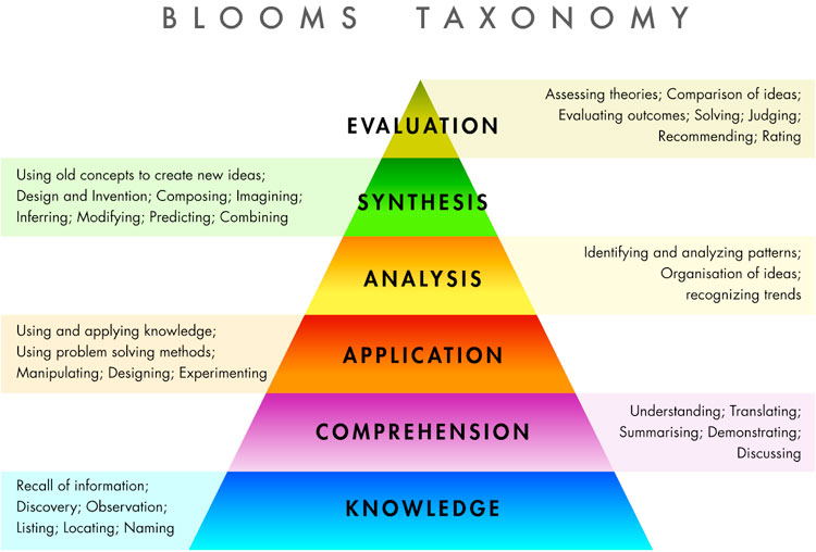
I'm in the middle of writing about various pedagogic theories for PCUTL (a higher education certification process) and I needed a picture of Bloom's taxonomy:
I needed to be able to play around with it a bit (so as to add annotations and colours like in the above picture) so I wanted something in Tikz. I found this helpful stack-exchange post for hierarchical pyramids and stole modified the code from there to get Bloom's taxonomy in Tikz. Here's the stripped down version:
In my previous post I posted a small python script that will recursively go through all directories in a directory and return the word count distribution using texcount (a utility that strips away LaTeX code to count words in documents). In this one I'm going to try and find a way of finding out how many words are in my LaTeX files without counting them (kind of).
On G+ +Dima Pasechnik suggested the use of wc as a proxy but wc gives the count of all words (include code words). I thought I'd see how far off wc would be. So I modified the python script from my last post so that it not only runs texcount but also wc and carries out a simple linear regression (using the stats package from scipy). The script is at the bottom of this blog post.
Here's the scatter plot and linear fit for all the LaTeX files on my system:
We see that the line $y=.68x-27.01$ can be accepted as a predictor for the number of words in a LaTeX document as a function of the total number of code words.
As in my previous post I obviously have an outlier there so here's the scatter plot and linear fit when I remove that one larger file:
The coefficient is again very similar $y=.64x+26$.
So based on this I'd say that multiplying the number of codewords in a .tex file by .6 is going to give me a good indication of how many words I have in total.
Here's a csv file with my data, I'd love to know if other people have similar fits.
So today I found out about latexcount which will give a nice detailed word count for LaTeX files. It's really easy to use and apparently comes with most LaTeX distributions (it was included with my TeXlive distribution under Mac OS and Linux).
To run it is as simple as:
$ texcount file.tex
It will output a nice detailed count of words (breaking down by sections etc...). I don't pretend to be an expert in anything but I'm genuinely really surprised that I had never seen this before. I was about to write a (most probably terrible) +Python script to count words in a given file and just before starting I thought "WAIT A MINUTE: someone must have done this"...
Anyway, I've gotten to the point of not being able to watch TV without a laptop at the tip of my fingers doing some type of work so whilst keeping an eye on South Africa playing ridiculously well in their win over Australia in the rugby championship I thought I'd see if I could have a bit of fun with texcount.
Here's a very simple Python script that will recursively search through all directories in a given directory and count the words in all the LaTeX files:
#!/usr/bin/env pythonimport fnmatch
import os
import subprocess
import argparse
import matplotlib.pyplot as plt
import pickle
def trim(t, p=0.01):
    """Trims the largest and smallest elements of t.

    Args:
    t: sequence of numbers
    p: fraction of values to trim off each end

    Returns:
    sequence of values
    """
    t.sort()
    n = int(p * len(t))
    t = t[n:-n]
    return t

parser = argparse.ArgumentParser(description="A simple script to find word counts of all tex files in all subdirectories of a target directory.")
parser.add_argument("directory", help="the directory you would like to search")
parser.add_argument("-t", "--trim", help="trim data percentage", default=0)
args = parser.parse_args()
directory = args.directory
p = float(args.trim)

matches = []
for root, dirnames, filenames in os.walk(directory):
  for filename in fnmatch.filter(filenames, '*.tex'):
        matches.append(os.path.join(root, filename))

wordcounts = {}
fails = {}
for f in matches:
    print "-" * 30
    print f
    process = subprocess.Popen(['texcount', '-1', f],stdout=subprocess.PIPE)
    out, err = process.communicate()
    try:
        wordcounts[f] = eval(out.split()[0])
        print "\t has %s words." % wordcounts[f]
    except:
        print "\t Couldn't count..."
        fails[f] = err

pickle.dump(wordcounts, open('latexwordcountin%s.pickle' % directory.replace("/", "-"), "w"))


try:
    data = [wordcounts[e] for e in wordcounts]
    if p != 0:
        data = trim(data, p)
    plt.figure()
    plt.hist(data, bins=20)
    plt.xlabel("Words")
    plt.ylabel("Frequency")
    plt.title("Distribution of words counts in all my LaTeX documents\n ($N=%s$,mean=$%s$, max=$%s$)" % (len(data), sum(data)/len(data), max(data)))
    plt.savefig('latexwordcountin%s.svg' % directory.replace("/", "-"))
except:
    print "Graph not produced, perhaps you don't have matplotlib installed..."
(Please forgive the lack of comments throughout the code...)
Here is what calls it on my entire Dropbox folder:
$ ./searchfiles.py ~/Dropbox
This will run through my entire Dropbox and count all *tex files (it threw up errors on some of my files so I have some error handling in there). It will output a dictionary of file name - word count pairs to a pickle (so you could do whatever you want with that) file but if you have matplolib installed it should also produce the following histogram:
As you can see from there it looks like I've got some files quite a lot bigger than the others (I'm guessing latexcount will count individual chapters as well as the entire thesis.tex files that I have in there that include them...). So I've added an option to trim the data set before plotting:
$ ./searchfiles.py ~/Dropbox -t .05
This takes 5% of the data off each side of our data set and gives:
Looking at that I have a lot of very short LaTeX files (which include some standalone images I've drawn to do stuff like this). If I had time I'd see how good a negative exponential fits to that distribution as it does indeed look kind of random. I'd love to see how others' word count distribution looks...
Now, I can say that if I ever produce more than 600 words then I'm doing above average work...

.png)
.png)

.png)

.png)
.png)