Pigeon holes, Markov chains and Sagemath.

On the 16/10/2013 I posted the following picture on G+:

Here's what I wrote on that post:

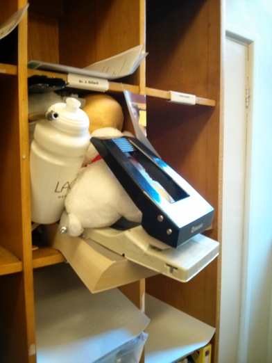
For a while now there's been a 'game' going on with our pigeon holes where people would put random objects in other people's pigeon holes (like the water bottle you see in the picture). These objects would then follow a random walk around the pigeon holes as each individual would find an object in their pigeon hole and absent-mindedly move it to someone else's pigeon hole.

As such each pigeon hole could be thought of as being a transient state in a Markov chain (http://en.wikipedia.org/wiki/Markov_chain). What is really awesome is that one of the PhD students here didn't seem to care when these random objects appeared in her pigeon hole. Her pigeon hole was in fact an absorbing state. This has now resulted in more or less all random objects (including a wedding photo that no one really knows the origin of) to be in her pigeon hole.

I thought I'd have a go at modelling this as an actual Markov chain. Here's a good video by a research student of mine (+Jason Young) describing the very basics of a Markov chain:

To model the movement of an object as a Markov chain we first of all need to describe the states. In our case this is pretty easy and we simply number our pigeon holes and refer to them as states. In my example there I've decided to model a situation with 12 pigeon holes.

What we now need is a set of transition probabilities which model the random behaviour of people finding an object in their pigeon hole and absent-mindedly moving it to another pigeon hole.

This will be in the form of a matrix $P$. Where $P_{ij}$ denotes the probability of going from state $i$ to state $j$.

I could sit in our photocopier room (that's where our pigeon holes are) and take notes as to where the individual who owns pigeon hole $i$ places the various objects that appear in their pigeon hole...
That would take a lot of time and sadly I don't have any time. So instead I'm going to use +Sage Mathematical Software System. The following code gives a random matrix:

N = 12
P = random_matrix(QQ, N, N)

This is just a random matrix over $\mathbb{Q}$ so we need to do tiny bit of work to make it a stochastic matrix:

P = [[abs(k) for k in row] for row in P]  # This ensures all our numbers are positive
P = matrix([[k / sum(row) for k in row] for row in P]) # This ensures that our rows all sum to 1

The definition of a stochastic matrix is any matrix $P$ such that:

• $P$ is square
• $P_{ij}\geq 0$ (all probabilities are non negative)
• $\sum_{j}P_{ij}=1\;\forall\;i$ (when leaving state $i$ the probabilities of going to all other states must sum to 1)

Recall that our matrix is pretty big (12 by 12) so we the easiest way to visualise it is through a heat map:

P.plot(cmap='hsv',colorbar=True)

Here's what a plot of our matrix looks like (I created a bunch of random matrix gifs here):

We can find the steady state probability of a given object being in any given state using a very neat result (which is not actually that hard to prove). This probability vector $\pi$ (where $\pi_i$ denotes the probability of being in state $i$) will be a solution of the matrix equation:

$$\pi P = \pi$$

To solve this equation it can be shown that we simply need to find the eigenvector of $P$ corresponding to the unit eigenvalue:

eigen = P.eigenvectors_left()  # This finds the eigenvalues and eigenvectors

To normalise our eigenvector we can do this:

pi = [k[1][0] for k in eigen if k[0] == 1][0]  # Find eigenvector corresponding to unit eigenvalue
pi = [k / sum(pi) for k in pi]  # normalise eigenvector

Here's a bar plot of out probability vector:

bar_chart(pi)

We can read the probabilities from this chart and see the probability of finding any given object in a particular pigeon hole. The bar_chart function in Sage still needs a bit of work and at the moment can only print a single list of data so it automatically has the axis indexed from 0 onwards (not from 1 to 12 as we would want). We can easily fix this using some matplotlib code (Sage is just wrapping matplotlib anyway):

import matplotlib.pyplot as plt

plt.figure()
plt.bar(range(1, N + 1), pi)
plt.savefig("betterbarplot.png")

Here's the plot:

We could of course pass a lot more options to the matplotlib plot to make it just as we want (and I'll in fact do this in a bit). The ability to use base python within Sage is really awesome.

One final thing we can do is run a little simulation of our objects going through the chain. To do this we're going to sample a sequence of states (pigeon holes $i$). For every $i$ we sample a random number $0\ r\leq 1$ and find $j$ such that $\sum_{j'=1}^{j}P_{ij'}. This is a random sampling technique called inverse random sampling.

import random

def nextstate(i, P):
    """
    A function that takes a transition matrix P, a current state i (assumingstarting at 0) and returns the next state j
    """
    r = random.random()
    cumulativerow = [P[i][0]]
    for k in P[i][1:]:  # Iterate through elements of the transition matrix
        cumulativerow.append(cumulativerow[-1] + k)  # Obtain the cumulative distribution
    for j in range(len(cumulativerow)):
        if cumulativerow[j] >= r:  # Find the next state using inverse sampling
            return j
    return j

states = [0]
numberofiterations = 1000
for k in range(numberofiterations):
    states.append(nextstate(states[-1],P))

We can now compare our simulation to our theoretical result:

import matplotlib.pyplot as plt

plt.figure()
plt.bar(range(1, N + 1), pi, label='Theory')  # Plots the theoretical results
plt.hist([k + 1 for k in states], color='red', bins=range(1, N + 2), alpha=0.5, normed=True, histtype='bar', label='Sim')  # Plots the simulation result in a transparent red
plt.legend()  # Tells matplotlib to place the legend
plt.xlim(1, N)  # Changes the limit of the x axis
plt.xlabel('State')  # Include a label for the x axis
plt.ylabel('Probability')  # Include a label for the y axis
plt.title("After %s steps" % numberofiterations)  # Write the title to the plot
plt.savefig("comparingsimulation.png")

We see the plot here:

A bit more flexing of muscles allows us to get the following animated gif in which we can see the simulation confirming the theoretical result:

This post assumes that all our states are transitive (although our random selection of $P$ could give us a non transitive state) but the motivation of my post is the fact that one of our students' pigeon holes was in fact absorbing. I'll write another post soon looking at that (in particular seeing which pigeon hole is most likely to move the object to the absorbing state).