Playing Stochastic/Markov games in class

In class on Monday my students and I looked at Stochastic games (Chapter 14 of my course notes). I decided to play a tournament similar to the iterated games that we played previously (corresponding to Chapters 9 and 10). I've blogged about them here and here.

In short, a stochastic game is a collection of states that themselves correspond to games. After players select strategies at a given state/game the next game they play (or state they are in) is given by a probability distribution.

This is a bit like playing in a casino where the table you play at depends on what happened at the previous table you played.

*The game we played in class corresponds to a casino with two tables:*

- At the first table we play a simple prisoner's dilemma (players aiming to maximise) their utility:

$$\begin{pmatrix}
(2,2)&(0,3)\\
(3,0)&(1,1)
\end{pmatrix}$$

The probability distribution at this table (indicating what game we played next) is given by:

$$\begin{pmatrix}
(.75,.25)&(0,1)\\
(0,1)&(.5,.5)
\end{pmatrix}$$

    - If both players cooperate (getting a utility of $2$ each) then there is a 75% chance that they play at this same table again.
    - If only one player cooperates and the other defects (the defector getting a utility of $3$ and the cooperator a utility of $0$) then the players move to the other game with 100% probability.
    - If both players defect (each getting a utility of $1$) then they will play the same game with 50% chance.

- The second table was a dummy game that basically ended the game:

$$\begin{pmatrix}
(0&0)
\end{pmatrix}$$

The probability distribution for this game is $(0,1)$.

The assumption made in this class is that the games are played infinitely and as such a discounting factor $\delta$ is used. When playing this in class we interpreted the discounting factor as the probability of the game continuing. So the game ended when the probabilities indicated that we were in the second game or when the discounting factor said so (we used $\delta=1/2$).

The class formed 4 teams and we played a round robin.

The first round had Tom's Team go up against Team Roy and Barmy go up against 4:

We see that Tom's team and Team Roy cooperated both times before the game ended whilst 4 defected from the start against Barmy.

The next round had Barmy go up against Tom's Team and Team Roy go up against 4:

We see that Barmy and Team Roy both cooperated before the game ended and Team Roy and 4 both defected before the game ended.

The last game had Tom's Team go up against 4 and Team Roy go up against Barmy. Below you can also see the final cumulative scores:

As you can see Tom's Team won (the name is after +Paul Harper son Tom joined the class during which we played the iterated prisonder's dilemma).

To decide who came second (they could choose the second prize to either be apples or party rings) a best of three game of Rock, Paper, Scissors, Lizard, Spock was played with Joe winning the party rings for Team Roy ('Scissors decapitates lizard').

I think this was good fun and hopefully enabled the students to have a sound grasp of what is meant by a state, a transition, etc..

Interestingly all teams happened to play Markov Strategies (i.e. in any given game they all did the same thing in each state) although this might have been different if the probabilities allowed the game to last longer. In the course we are restricting ourselves to Markov strategies.

After playing this we went through obtaining 2 equilibria for this game (both players defecting and both players cooperating).

Here are some photos that a student grabbed during the class and also a re-share of the gif of +Paul Harper's son Tom using a Nerf gun on those who defected against his team during the Prisoner's dilemma tournament:

Pigeon holes, Markov chains and Sagemath.

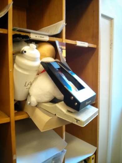
On the 16/10/2013 I posted the following picture on G+:

Here's what I wrote on that post:

For a while now there's been a 'game' going on with our pigeon holes where people would put random objects in other people's pigeon holes (like the water bottle you see in the picture). These objects would then follow a random walk around the pigeon holes as each individual would find an object in their pigeon hole and absent-mindedly move it to someone else's pigeon hole.

As such each pigeon hole could be thought of as being a transient state in a Markov chain (http://en.wikipedia.org/wiki/Markov_chain). What is really awesome is that one of the PhD students here didn't seem to care when these random objects appeared in her pigeon hole. Her pigeon hole was in fact an absorbing state. This has now resulted in more or less all random objects (including a wedding photo that no one really knows the origin of) to be in her pigeon hole.

I thought I'd have a go at modelling this as an actual Markov chain. Here's a good video by a research student of mine (+Jason Young) describing the very basics of a Markov chain:

To model the movement of an object as a Markov chain we first of all need to describe the states. In our case this is pretty easy and we simply number our pigeon holes and refer to them as states. In my example there I've decided to model a situation with 12 pigeon holes.

What we now need is a set of transition probabilities which model the random behaviour of people finding an object in their pigeon hole and absent-mindedly moving it to another pigeon hole.

This will be in the form of a matrix $P$. Where $P_{ij}$ denotes the probability of going from state $i$ to state $j$.

I could sit in our photocopier room (that's where our pigeon holes are) and take notes as to where the individual who owns pigeon hole $i$ places the various objects that appear in their pigeon hole...
That would take a lot of time and sadly I don't have any time. So instead I'm going to use +Sage Mathematical Software System. The following code gives a random matrix:

N = 12
P = random_matrix(QQ, N, N)

This is just a random matrix over $\mathbb{Q}$ so we need to do tiny bit of work to make it a stochastic matrix:

P = [[abs(k) for k in row] for row in P]  # This ensures all our numbers are positive
P = matrix([[k / sum(row) for k in row] for row in P]) # This ensures that our rows all sum to 1

The definition of a stochastic matrix is any matrix $P$ such that:

• $P$ is square
• $P_{ij}\geq 0$ (all probabilities are non negative)
• $\sum_{j}P_{ij}=1\;\forall\;i$ (when leaving state $i$ the probabilities of going to all other states must sum to 1)

Recall that our matrix is pretty big (12 by 12) so we the easiest way to visualise it is through a heat map:

P.plot(cmap='hsv',colorbar=True)

Here's what a plot of our matrix looks like (I created a bunch of random matrix gifs here):

We can find the steady state probability of a given object being in any given state using a very neat result (which is not actually that hard to prove). This probability vector $\pi$ (where $\pi_i$ denotes the probability of being in state $i$) will be a solution of the matrix equation:

$$\pi P = \pi$$

To solve this equation it can be shown that we simply need to find the eigenvector of $P$ corresponding to the unit eigenvalue:

eigen = P.eigenvectors_left()  # This finds the eigenvalues and eigenvectors

To normalise our eigenvector we can do this:

pi = [k[1][0] for k in eigen if k[0] == 1][0]  # Find eigenvector corresponding to unit eigenvalue
pi = [k / sum(pi) for k in pi]  # normalise eigenvector

Here's a bar plot of out probability vector:

bar_chart(pi)

We can read the probabilities from this chart and see the probability of finding any given object in a particular pigeon hole. The bar_chart function in Sage still needs a bit of work and at the moment can only print a single list of data so it automatically has the axis indexed from 0 onwards (not from 1 to 12 as we would want). We can easily fix this using some matplotlib code (Sage is just wrapping matplotlib anyway):

import matplotlib.pyplot as plt

plt.figure()
plt.bar(range(1, N + 1), pi)
plt.savefig("betterbarplot.png")

Here's the plot:

We could of course pass a lot more options to the matplotlib plot to make it just as we want (and I'll in fact do this in a bit). The ability to use base python within Sage is really awesome.

One final thing we can do is run a little simulation of our objects going through the chain. To do this we're going to sample a sequence of states (pigeon holes $i$). For every $i$ we sample a random number $0\ r\leq 1$ and find $j$ such that $\sum_{j'=1}^{j}P_{ij'}. This is a random sampling technique called inverse random sampling.

import random

def nextstate(i, P):
    """
    A function that takes a transition matrix P, a current state i (assumingstarting at 0) and returns the next state j
    """
    r = random.random()
    cumulativerow = [P[i][0]]
    for k in P[i][1:]:  # Iterate through elements of the transition matrix
        cumulativerow.append(cumulativerow[-1] + k)  # Obtain the cumulative distribution
    for j in range(len(cumulativerow)):
        if cumulativerow[j] >= r:  # Find the next state using inverse sampling
            return j
    return j

states = [0]
numberofiterations = 1000
for k in range(numberofiterations):
    states.append(nextstate(states[-1],P))

We can now compare our simulation to our theoretical result:

import matplotlib.pyplot as plt

plt.figure()
plt.bar(range(1, N + 1), pi, label='Theory')  # Plots the theoretical results
plt.hist([k + 1 for k in states], color='red', bins=range(1, N + 2), alpha=0.5, normed=True, histtype='bar', label='Sim')  # Plots the simulation result in a transparent red
plt.legend()  # Tells matplotlib to place the legend
plt.xlim(1, N)  # Changes the limit of the x axis
plt.xlabel('State')  # Include a label for the x axis
plt.ylabel('Probability')  # Include a label for the y axis
plt.title("After %s steps" % numberofiterations)  # Write the title to the plot
plt.savefig("comparingsimulation.png")

We see the plot here:

A bit more flexing of muscles allows us to get the following animated gif in which we can see the simulation confirming the theoretical result:

This post assumes that all our states are transitive (although our random selection of $P$ could give us a non transitive state) but the motivation of my post is the fact that one of our students' pigeon holes was in fact absorbing. I'll write another post soon looking at that (in particular seeing which pigeon hole is most likely to move the object to the absorbing state).

Some analysis of the game shut the box

This Christmas, +Zoe Prytherch and I got my mother a small board game called: "Shut the Box" (also known as "Tric-Trac", "Canoga", "Klackers", "Zoltan Box", "Batten Down the Hatches", or "High Rollers" according to the wiki page). It's a neat little game with all sorts of underlying mathematics.

Here's a picture of us playing:

Here's a close up of the box:

A good description of the game can be found on the wiki page but basically the game can be described as follows:

• It is a Solitaire game that can be played in turns and scores compared (but no strategies arise due to interactions of players).
• The aim is to "shut" as many tiles (each being one of the digits from 1 to 9) as possible.
• On any given go, a player rolls two dice and/or has a choice of rolling one dice if the tiles 7,8,9 are "shut".
• The sum total of the dice roll indicates the sum total of tiles that must be "shut". If I roll 11, I could put down [2,9],[3,8],[1,2,8] etc...
• The game ends when a player can't "shut" tiles corresponding to the dice roll (including the case when all tiles are "shut").

Here's a plot of a game we played with a few of my mother's friends:

You can see that myself and Jean did fairly poorly while Zoë made the difference just at the end to win :)

The game could be modelled as a Markov decision process but over the past few days I decided to code it in Sage and investigate whether or not I could find out anything cool with regards to strategies. If you're not aware of Sage I thoroughly recommend you taking a look, it's an awesome open source mathematics package. In this instance I used the Partitions function to rapidly obtain various combinations of dice rolls and/or tile options to get the results I wanted.

The code is all in a github repo and I feel I've written an ok README file explaining how it works so if you're interested in playing with it please do! The code basically has two parts, the first allows you to play using the program instead of a game board (with prompts telling you what your available plays are).

Here's a quick screencast of me demonstrating some of the code:

The second part of the code allows for strategies to be written that play the game automatically ("autoplay"). I've considered 4 strateges:

• Random (Just randomly pick any potential tile combination)
• Shortest (Choose the tile combination that has shortest length: i.e. [3] instead of [1,2] ~ in case of a tie pick randomly)
• Longest (Choose the tile combination that has longest length: i.e. [1,2] instead of [3] ~ in case of a tie pick randomly)
• Greedy. This chooses the tile combination that ensures the best possible chance of the game not ending on the next go. This is calculated by summing the probabilities of obtaining a dice roll that could be obtained.

I've been leaving my computer run the code in the background for a while now so here are some early results. I've got over 90000 instances for Greedy and Random with over 40000 instances for the other two which I thought of later (EDIT: I know have over 400000 instances...). I've collected (as and when one of my home boxes was ideal) more data since writing this and the file is available for anyone to play with here. If I've made any mistakes with my analysis, I'd love to hear it!.

First of all what does the average score look like:

Greedy_Score   Random_Score     Longest_Score   Shortest_Score  
Min.   : 0.00  Min.   : 0.00    Min.   : 0.00   Min.   : 0.00  
1st Qu.: 6.00  1st Qu.:14.00    1st Qu.:18.00   1st Qu.: 7.00   
Median :11.00  Median :21.00    Median :24.00   Median :11.00
Mean   :11.42  Mean   :20.45    Mean   :24.16   Mean   :12.06  
3rd Qu.:16.00  3rd Qu.:27.00    3rd Qu.:30.00   3rd Qu.:17.00  
Max.   :43.00  Max.   :43.00    Max.   :43.00   Max.   :43.00  

Shortest and Greedy seem to do a fair bit better then the other two. If we take a look at the distribution of the scores that is confirmed:

If we also take a look at the length of the game (i.e. how many total dice rolls there were):

Greedy_Length  Random_Length  Longest_Length  Shortest_Length
Min.   :1.000  Min.   :1.000  Min.   :1.00    Min.   :1.00    
1st Qu.:4.000  1st Qu.:3.000  1st Qu.:2.00    1st Qu.:4.00    
Median :5.000  Median :3.000  Median :3.00    Median :5.00    
Mean   :4.897  Mean   :3.414  Mean   :2.86    Mean   :4.82    
3rd Qu.:6.000  3rd Qu.:4.000  3rd Qu.:4.00    3rd Qu.:6.00    
Max.   :9.000  Max.   :9.000  Max.   :8.00    Max.   :9.00    
                                                             

We see that games last longer when using Greedy and Shortest. If we look at the distribution we see (I've updated this graph since first publishing this post):

It looks like Greedy might allow for slightly longer games than Shortest. Whether or not playing Shortest or Greedy is actually any different seems interesting. A simple analysis of variance (ANOVA) seems to indicate that there is a significant effect:

Df  Sum Sq Mean Sq F value P

stbaov$Method      1   11337   11337   196.3 2e-16 

Residuals     127169 7345725      58

This is all experimental of course and analysing whether or not my suggested greedy strategy is indeed the optimal strategy would require some markov decision process modelling. I might look in to this with an undegraduate project student next year.

The tricky part about using the greedy method whilst actually playing the game with friends is that it requires a fair bit of calculation. Nothing that Sage can't handle in a split second but something that could keep people waiting a fair bit if you were to work it out with a pen and paper. Despite the significant statistical difference between the methods this analysis seems to indicate that choosing the shortest set of tiles is a pretty good strategy so if in doubt I recommend choosing that...

If anyone cares enough about all this to fork the code or suggest a different strategy I'd be delighted :) In case you missed it above, here's the github repo:

https://github.com/drvinceknight/Shut_The_Box

(On a technical note some of the pre analysis is done using python and the actual graphs seen here are done using R)