Debugging Python with pdb at the command line

I've just put up a short video (7 mins) describing one way of debugging in Python using the pdb module (here's the docs):

In this video I show how to step through code, view values of variables and also insert various types of break points.

All this is done interactively at the command line but you can also use the pdb library to include debugging commands in your Python script itself.

My students write about their first Python conference

Last week I wrote about my impressions from my first Open Source Software conference (OSS): https://djangoweekend.org/

It was an awesome conference but the highlight for me was seeing 3 of my students take full advantage of the event. I asked Matt, Alex and James to write a bit of a guest post for this blog about their experiences:

--------------------------------

Here's what Matt had to say:

"Having never been to a conference like this before, and with only a few months of coding experience under my belt, I had no idea what to expect from Django Weekend Cardiff. Despite this I had an incredible weekend. Everyone that I met and talked to was friendly and more than willing to answer my questions. 

While some of the talks went a little over my head, the clinics were very helpful in getting me started with Django. I even felt confident enough to give a lightning talk, that gave me the chance to voice my opinion on computing with regards to education, and how it had helped me over the few months I was leaning it as part of my undergraduate course for maths.


Overall I had a great time, and will definitely be keeping an eye out for Django Weekend Cardiff 2015."

Matt's lightning talk was recorded so as soon as it's online I will be post about it. He did an awesome job.

--------------------------------

Here's what +Alex Carney had to say:

"I first became aware of the open source scene when I was in Year 7 and my dad installed Ubuntu 7.10 on my ancient laptop in a bid to keep it usable. I slowly became more and more fascinated on what software I was able to download for free and have a play with, from creating animations with Blender to messing around in GIMP and to hear him say that it was made by normal people such as ourselves I was blown away thinking how on Earth could people like my dad and myself create such wonders?

Well needless to say it reignited my desire to learn programming, I had dabbled with Pascal and BASIC beforehand but I couldn't get much further than a series of print statements and lost interest. But then to discover Python, a language with syntax that was actually readable to someone just starting secondary school was amazing, slowly I was able to teach myself parts of it in short bursts over the years, before dropping it when I was in Year 11, to learn C++ mostly forgetting about Python.

Fast forward to September 2013, when I started my Maths degree at Cardiff Uni, and I finding out that I would be taught Python as part of the course was like being reunited with an old friend. But this time there was a major difference I was actually using Python. Back when I was teaching myself I never had any concrete goals or deadlines, I would follow one example before swiftly moving on to the next without stopping to apply what I had learnt. So naturally it was hard to maintain focus and I never produced anything worthwhile. 

However being set tasks to complete was great as I was finally applying my knowledge I had gained over the years and was able to appreciate how useful being able to program is, once you start thinking like a programmer the only limit is your imagination - Oh! and of course how powerful your computer is...

I can't thank Vince and the School of Mathematics at Cardiff enough for sponsoring me to go to the conference because it made me realise a lot of things. Firstly is that there really is a thriving welcoming community on the open source scene. I was always vaguely aware that it existed as I trawled through forums and mailing lists looking for solutions to problems I was having, but something always stopped me from joining in. I was thinking that even though it was open there was some mystical entry barrier that you had to pass before you would be accepted.

However by going to the conference I was shown the complete opposite. Nobody so much batted an eyelid when they saw me, some student only just able to scratch the surface of Python's power and knowing absolutely nothing about Django. Moreover they wanted to speak to me, they wanted to hear about it from a beginner's perspective, they wanted to know what it was like learning Django for the first time, what could they do to make it easier for me to learn? While having a chat with one of the core Django developers I pointed out that I didn't find certain steps in a tutorial that clear and afterwards he went away and amended the tutorial clearing up the confusion that I had!

It was incredibly interesting to hear how other people have used Python in their work and I was blown away at the power of not only the programming language itself but the community as well. An example from a particular talk was the Astronomy community, how Python was able to help the community create a common standard for sharing data and how all the tools developed by individuals went on to benefit the community as a whole. Leaving researchers able to concentrate more on the science than the technical difficulties and headaches of having to deal with fragmented standards and datasets.

I want to finish by saying how truly inspired attending the conference made me and I not only want to thank Vince and the School of Mathematics for giving me the opportunity, but to thank Daniele Procida for making the conference a reality in the first place. I will definitely want to attend next year's and I'm even thinking of going to  PyConUK in September. I am yet to contribute to an open source project but I'm hoping that's an issue I can fix sooner rather than later."

Alex was one of the students in the class with the most starting knowledge; in fact he helped me win a bet with +Jason Young (that I would be able to get a student to use Vim before the end of the year: Alex used Vim from the start...). It's really nice to read that he found the whole conference interesting and more importantly inspiring.

--------------------------------

The final post is from +James Campbell but he has his own blog that I'd really recommend you taking a look at (James is also a rugby referee so he blogs about that as well). Here's the post he wrote about the conference: http://www.jamescampbell.org.uk/?p=417

If it's too much effort to click over to there here's a bit I stole:

"Today they were working on fixing bugs and reviewing code for the upcoming Django 1.7 release. However, despite how busy they were, whenever I needed a hand someone was happy to help. At one point I had Django core developers discussing the best way to solve one of my problems. These guys are some of the best in the world at what they do, yet they still found time to help a complete newcomer, and I’m really grateful to all those who did so."

My students and my first PyCon

A couple of months ago an email somehow found it's way in to my inbox mentioning a new user group that was setting up in Cardiff. This was from some guy called Daniele Procida. As a Python coder really enthusiastic to be part of the Open Source Software (OSS) community I thought this would be awesome so I've been along to the monthly meetings where all things Python and Django are discussed.

However many months later I got to attend my first PyCon (in fact a DjangoCon): https://djangoweekend.org/

Here's the programme that I carried around in my back pocket:

Professor Tim Phillips, the head of the School of Mathematics kindly agreed to sponsor 3 tickets for students on my Computing for Mathematics course. I gave 3 tickets to students as a reward for their individual coursework (James wrote about Markov chains and Snakes and Ladders, Alex about Fractals and Matt about prime numbers).

+Jason Young who has been my research undergraduate student for a couple of years now (and is a very able coder) attended and +Izabela Komenda (a post-doc) also presented some of her PhD work.

Here's a picture of my Cardiff students, Daniele and I:

It was great that so many sponsors contributed to the conference (full list here) and also that +Cardiff University supported the event wholeheartedly, Roger Whitaker (the dean of research for the physical sciences) even opened the scientific talks on Friday.

Frankly:

It was the best conference I've ever been to.


The atmosphere cultivated by the OSS community is really amazing. Everyone is really encouraging, understanding and just plain ol' nice.

From the scientific talks on the Friday where usages for Python in Science were discussed to witnessing what a 'code sprint' was on the Sunday: everyone was just exceptionally nice.

I learnt Django over christmas and the help people were willing to give (not once making my mistakes more than they were) was really cool.

For example this morning I sat down with Baptiste, one of the core Django developers and he really kindly answered all the (noobish) questions I had (before leaving today he actually gave me his card and told me to get in touch if I had any further problems with a particular thing).

That is just one example of the awesome atmosphere that was cultivated during the conference. The event brilliantly mixed advanced programming for one of the most popular web frameworks with accessible topics for every attendee. I think that this is something that is kind of inherent to the OSS community, you are encouraged to put yourself out there and potentially make mistakes.

For this reason alone I'm extremely glad that the 3 undergraduates got to attend the event. 

Fear of failure and mistakes is something that sometimes really holds students back. As educators it's very important for us to make sure students learn to embrace mistakes.

During one of the talks on Saturday a particular particularity of Django was being discussed and I thought to myself:

I wonder if my students will be put off by "how much they don't understand" and perhaps this will end up being a negative experience for them...

I could not have been more wrong, their attitudes were perfect. They realised that they were very much at the beginning of the road (some of them had not coded before October) and just took advantage of everything around them.

James gave a talk on the Friday which was great and Matt gave a lightning talk (less than 5mins):

They all spoke to the experts around them constantly and by Sunday were themselves writing Django apps. It was great to have +Robert Dragan of learnium help some of them debug their code on the Sunday.

In fact towards the end of Sunday James even had Daniele (a core Django developer) and Charlie (a super-duper really helpful and nice Django developer/person) helping him work on a site:

I won't write much more about the whole event but I'll just repeat something that Matt said during his lightning talk.

He started by saying that he was a bit dismayed when at the beginning of his degree he was told that he was going to have to learn how to code (my course is brand new), he then talked about how he thought +Sage Mathematical Software System helped him gain a better understanding of the prime number theorem but it was what he said last that was really awesome (a lot of other attendees commented on it):

"Why did I have to wait until coming to University to learn to code?"

(All the talks on Saturday were recorded so I really look forward to sharing his talk, it was very well delivered.)

This whole event was a really great experience for me but more importantly my students.

The conference will be running again next here which is awesome for my future students. Next time Daniele, (who is one of the most impressive human beings I've ever met) will have (at least) me to help organise the it.

I've already signed up for my next PyCon (http://pyconuk.org/) and more importantly I've asked myself:

"Why did I have to wait till now to attend an OSS conference?"

What happens when I ask students if they have seen 'A Beautiful Mind'

For the past 4~5 years now I've been lucky enough to tag along with +Paul Harper when he does outreach in high schools. I've developed my own little 'roadshow' that introduces students to Game Theory.

On Wednesday there was a cool event at the School of Mathematics where we had 120 odd 17 year olds in to get a taste for the Mathematics at University (some pics: here and here).

I've blogged many times (and +Dana Ernst has as well: here) about the activity that I run which involves a Prisoners dilemma tournament and 2 rounds of a 2/3rds of the average game, here is my updated set of results over all the times I've played it (the second guess is after we all discuss rational behaviour):

(if any of my student are reading this the above could help them win a box of chocolates on Monday)

This is not the purpose of this post.

Something terrible happened on Wednesday.

During my activity I always show this clip from A Beautiful Mind (awesome movie about John Nash):

Before showing the clip I always ask: "How many of you have seen the movie 'A Beautiful Mind'?".

Now, I've been doing this for 4~5 years and the response I get to this question has made me realise that I'm not cool anymore. I guess there's a point in everyone's life where that realisation hits them. I've been in denial until Wednesday when for the first time ever: not one student had seen the movie :'(. This makes me sad because I think this is probably one of my favourite movies and one I've always thought was pretty cool.

Here's a little plot showing what I've been telling myself over the past few years (the fact that xkcd style graphs is now native to matplotlib is cool, my previous attempt at one of these: 'probability of saying yes to academic responsabilities'):

When I first asked and had about a quarter of the room know what I was talking about I thought that it was kind of cool and a sign of no longer being a kid...

When in twenty years time I embarrass my daughter by opening the door to her boyfriend/girlfriend wearing pyjamas; inviting him/her inside for a talk and reading him/her passages of my PhD thesis or whatever else I can think of, I'll be able to say that it's revenge for not being cool any more and that I made this decision on the 22nd of January 2014.

Plotting complex numbers in Sage

I had a student email me overnight asking how to plot complex numbers in +Sage Mathematical Software System.

I spent a couple of minutes googleing and found various command that would plot complex functions:

f = sqrt(x) + 1 / x complex_plot(sqrt, (-5,5), (-5, 5))

This gives the following plot:

This was however not what my student was asking. They wanted to know how to plot a given set of points in the complex plain (referred to as the Argand plane). A quick google to check if there was anything in Sage pre built for this brought me to this published sheet by +Jason Grout.

I tweaked it slightly so that it was in line with the commands my students have learnt so far and also to include axes legends and put the following in to a function:

def complex_point_plot(pts): 
    """ 
    A function that returns a plot of a list of complex points. 
    Arguments: pts (a list of complex numbers) 
    Outputs: A list plot of the imaginary numbers 
    """ 
    return list_plot([(real(i), imag(i)) for i in pts], axes_labels = ['Re($z$)', 'Im($z$)'], size=30)

This function simply returns a plot as required. Here is a small test with the output:

complex_point_plot([3*I, e^(I*pi), e^(I*3*pi/4), 4-4*I])




Here is some code that will plot the unit circle using the $z=e^{i\theta}$ notation for complex numbers (and the Sage srange command):

pts = [e^(I*(theta)) for theta in srange(0, 2*pi, .1)] 
complex_point_plot(pts) 


Here is the output:

I published all this in a worksheet on our server so it's now immediately available to all our students. I'm really enjoying teaching +Sage Mathematical Software System to our students.

A Sage cell with the above code (that you can run in your browser) can be found here: http://goo.gl/jipzxV

EDIT: Since posting this +Punarbasu Purkayastha pointed out on G+ that list_plot can handle complex points right out of the box :) So the above can just be obtained by typing:

pts = [e^(I*(theta)) for theta in srange(0, 2*pi, .1)] 

list_plot(pts, axes_labels=['Re($z$)','Im($z$)'], size=30)

Learn something new everyday...

Selfish behaviour in queues and some open source graphical simulation software

In 1969 Naor, wrote a really nice paper called 'The Regulation of Queue Size by Levying Tolls'. In this paper Naor considered a system with a single server queue:

• With an arrival rate $\lambda$ (customers per time unit)
• A service rate $\mu$ (customers per time unit)
• and a reward and cost for service that can actually just be considered as a "value for service": $\beta$

Naor then considered two types of customers: Selfish and Optimal.

It is relatively straightforward to see that Selfish customers should join if and only if:

$$\frac{n+1}{\mu}\leq \beta$$

where $n$ is the number of other customers in the system upon arrival.

What is slightly less straightforward is that Optimal customers should join if and only if $n\leq n^*$ where:

\[\frac{n^*(1-\rho)-\rho(1-\rho^{n^*})}{(1-\rho)^2}\leq \beta \mu < \frac{(n^*+1)(1-\rho)-\rho(1-\rho^{n^*+1})}{(1-\rho)^2}\]

(where $\rho=\lambda/\mu$)

It's a really cool result and one that has given rise to a lot more research (including what I mainly enjoy looking at).

I was asked recently be a colleague to give a 15 minute talk about my research to her second year OR class who will have just seen some queueing theory. I decided to talk about Naor's paper and thought that it would be nice if I could give a graphical representation of the customers arriving at the queue (similar to the DES package: +SIMUL8). So I spent some time writing a simulation engine and using the in built +Python Turtle library to get some graphics. A part from some of the optional plotting (matplotlib), this only uses base python libraries. Here's a gif from an early prototype:

Here's a video discussing Naor's result and showing demonstrating everything with my simulation model:

The code is all up on github and it really could do with some improving so it would be great if anyone wanted to contribute: https://github.com/drvinceknight/Simulating_Queues

Pigeon holes, Markov chains and Sagemath.

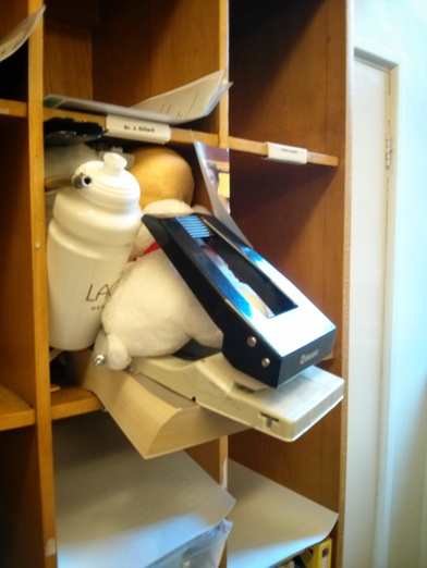
On the 16/10/2013 I posted the following picture on G+:

Here's what I wrote on that post:

For a while now there's been a 'game' going on with our pigeon holes where people would put random objects in other people's pigeon holes (like the water bottle you see in the picture). These objects would then follow a random walk around the pigeon holes as each individual would find an object in their pigeon hole and absent-mindedly move it to someone else's pigeon hole.

As such each pigeon hole could be thought of as being a transient state in a Markov chain (http://en.wikipedia.org/wiki/Markov_chain). What is really awesome is that one of the PhD students here didn't seem to care when these random objects appeared in her pigeon hole. Her pigeon hole was in fact an absorbing state. This has now resulted in more or less all random objects (including a wedding photo that no one really knows the origin of) to be in her pigeon hole.

I thought I'd have a go at modelling this as an actual Markov chain. Here's a good video by a research student of mine (+Jason Young) describing the very basics of a Markov chain:

To model the movement of an object as a Markov chain we first of all need to describe the states. In our case this is pretty easy and we simply number our pigeon holes and refer to them as states. In my example there I've decided to model a situation with 12 pigeon holes.

What we now need is a set of transition probabilities which model the random behaviour of people finding an object in their pigeon hole and absent-mindedly moving it to another pigeon hole.

This will be in the form of a matrix $P$. Where $P_{ij}$ denotes the probability of going from state $i$ to state $j$.

I could sit in our photocopier room (that's where our pigeon holes are) and take notes as to where the individual who owns pigeon hole $i$ places the various objects that appear in their pigeon hole...
That would take a lot of time and sadly I don't have any time. So instead I'm going to use +Sage Mathematical Software System. The following code gives a random matrix:

N = 12
P = random_matrix(QQ, N, N)

This is just a random matrix over $\mathbb{Q}$ so we need to do tiny bit of work to make it a stochastic matrix:

P = [[abs(k) for k in row] for row in P]  # This ensures all our numbers are positive
P = matrix([[k / sum(row) for k in row] for row in P]) # This ensures that our rows all sum to 1

The definition of a stochastic matrix is any matrix $P$ such that:

• $P$ is square
• $P_{ij}\geq 0$ (all probabilities are non negative)
• $\sum_{j}P_{ij}=1\;\forall\;i$ (when leaving state $i$ the probabilities of going to all other states must sum to 1)

Recall that our matrix is pretty big (12 by 12) so we the easiest way to visualise it is through a heat map:

P.plot(cmap='hsv',colorbar=True)

Here's what a plot of our matrix looks like (I created a bunch of random matrix gifs here):

We can find the steady state probability of a given object being in any given state using a very neat result (which is not actually that hard to prove). This probability vector $\pi$ (where $\pi_i$ denotes the probability of being in state $i$) will be a solution of the matrix equation:

$$\pi P = \pi$$

To solve this equation it can be shown that we simply need to find the eigenvector of $P$ corresponding to the unit eigenvalue:

eigen = P.eigenvectors_left()  # This finds the eigenvalues and eigenvectors

To normalise our eigenvector we can do this:

pi = [k[1][0] for k in eigen if k[0] == 1][0]  # Find eigenvector corresponding to unit eigenvalue
pi = [k / sum(pi) for k in pi]  # normalise eigenvector

Here's a bar plot of out probability vector:

bar_chart(pi)

We can read the probabilities from this chart and see the probability of finding any given object in a particular pigeon hole. The bar_chart function in Sage still needs a bit of work and at the moment can only print a single list of data so it automatically has the axis indexed from 0 onwards (not from 1 to 12 as we would want). We can easily fix this using some matplotlib code (Sage is just wrapping matplotlib anyway):

import matplotlib.pyplot as plt

plt.figure()
plt.bar(range(1, N + 1), pi)
plt.savefig("betterbarplot.png")

Here's the plot:

We could of course pass a lot more options to the matplotlib plot to make it just as we want (and I'll in fact do this in a bit). The ability to use base python within Sage is really awesome.

One final thing we can do is run a little simulation of our objects going through the chain. To do this we're going to sample a sequence of states (pigeon holes $i$). For every $i$ we sample a random number $0\ r\leq 1$ and find $j$ such that $\sum_{j'=1}^{j}P_{ij'}. This is a random sampling technique called inverse random sampling.

import random

def nextstate(i, P):
    """
    A function that takes a transition matrix P, a current state i (assumingstarting at 0) and returns the next state j
    """
    r = random.random()
    cumulativerow = [P[i][0]]
    for k in P[i][1:]:  # Iterate through elements of the transition matrix
        cumulativerow.append(cumulativerow[-1] + k)  # Obtain the cumulative distribution
    for j in range(len(cumulativerow)):
        if cumulativerow[j] >= r:  # Find the next state using inverse sampling
            return j
    return j

states = [0]
numberofiterations = 1000
for k in range(numberofiterations):
    states.append(nextstate(states[-1],P))

We can now compare our simulation to our theoretical result:

import matplotlib.pyplot as plt

plt.figure()
plt.bar(range(1, N + 1), pi, label='Theory')  # Plots the theoretical results
plt.hist([k + 1 for k in states], color='red', bins=range(1, N + 2), alpha=0.5, normed=True, histtype='bar', label='Sim')  # Plots the simulation result in a transparent red
plt.legend()  # Tells matplotlib to place the legend
plt.xlim(1, N)  # Changes the limit of the x axis
plt.xlabel('State')  # Include a label for the x axis
plt.ylabel('Probability')  # Include a label for the y axis
plt.title("After %s steps" % numberofiterations)  # Write the title to the plot
plt.savefig("comparingsimulation.png")

We see the plot here:

A bit more flexing of muscles allows us to get the following animated gif in which we can see the simulation confirming the theoretical result:

This post assumes that all our states are transitive (although our random selection of $P$ could give us a non transitive state) but the motivation of my post is the fact that one of our students' pigeon holes was in fact absorbing. I'll write another post soon looking at that (in particular seeing which pigeon hole is most likely to move the object to the absorbing state).

Just over two years with linux and the terminal: some thoughts and a plugin-less vimrc

So two years ago I decided to find out what linux was. Here's my first post on +Google+ 'announcing' that I was going all in and asking for some tips:

At the time I had some comments about using vim to modify my .bashrc. I politely thanked people saying that I'd look in to it and having absolutely no idea what was going on.

After a couple of weeks I had worked really hard to get a system that gave me everything that my work Windows machine did (office working, LaTeX gui setup etc). At that point I remember speaking to a friend of mine that was a hardened linux user saying: "ok, I've not lost anything since moving from Windows but what's the point? What have I gained?". My friend didn't really give me a satisfactory answer but I quite enjoy being out of my comfort zone so I kept with it.

After a couple more weeks I began to see that a big  point is the community. For anything I wanted help with I could find some people who had done it before and timidly open up this voodoo-black-magic thing called the "terminal" and paste in some code that would fix whatever needed fixing.

So at that point I thought the point was:

• It's free;
• Don't lose anything;
• Gain a community

After a couple of months of scarily copying things in to the terminal and hearing people talk about 'scripting' and various other things I thought: "Right let's give the terminal a go". So I learnt vi(m). This is old but still amuses me:

That took me a while and I was ridiculously slow at first, basically staying away from anything but insert mode and slowly learning a few new commands every now and then.

I also began to understand the point of scripting and what the "terminal" is. I now script more or less everything I do, find myself typing ':wq' in my gmail window all the time, love git and pretty much sigh every time there's a particular thing that I need to do using my mouse and a gui.

The efficiency with which I can do stuff in the terminal is completely incomparable to how I worked before. I'm still very much an amateur but I really do love the terminal (I only learnt the other day that you can middle click to paste anything that is highlighted: that blew my mind).

I realise now that the point with linux is that I don't think I was really using a computer to it's full potential before, I was just using some stuff that people had put in place for me to do some stuff (there's nothing really wrong with that, it's just a bit constraining)... I'm again in no way an expert and there's so much I still can't wait to learnt (I ticked symbolic links of the list a couple of days ago). 

The other point I think with the terminal this time (and more generally with being comfortable outside of a GUI) is that there's so much amazing software out there that does ridiculous stuff but that does not have a GUI (one reason being how long it takes to make the d**n things).

Another great thing with forcing myself to get to know linux is that I can also use all the relevant skills on a Mac. My workflow is basically a browser for my gmail and a terminal for vim so I am really happy on either machine (I prefer my linux box for the ease of getting things exactly the way I like them, while my work machines have some commercial software that I occasionally need when I get particular types of email attachments and my Imac is quite possibly the prettiest thing I've ever seen). I hear that with powershell and cygwin and things like that you can almost get a Windows box in the same shape but I can't say I see myself wanting to try that.

Using any machine becomes extremely simple. Ssh'ing in to a server is a very comfortable thing to do as all I really need is vim. To make that a bit more comfortable I've put my vimrc up on github so I can just clone that and basically be at home anywhere. Here's a bit more about my vimrc:

A basic vimrc

I really fell in love with vim about a year ago after watching +Martin Brochhaus's talk showing how to turn vim into a +Python IDE:

After watching the talk I immediately rushed off to get pathogen setup and got the various plugins Martin mentioned working. It was awesome: my vim experience with Python was ridiculously awesome. I rushed to find a bunch of LaTeX plugins and I was pretty much complete.

I've decided now though that I want to understand those things a bit better so I'm going to start from a much more basic vimrc (just with some aliases and what not) and slowly pick and choose plugins bit by bit making sure I completely understand what they do.

That vimrc is here (it's based on a bunch of stuff from the basic parts of Martin's vimrc which you can find here).

I've put this up on github in a repository I plan on growing. I've also written a simple python script that creates a symbolic link in the home directory so that I just need to keep the repositories synced on all my machines and it'll all just work. In future that python scipt will check if pathogen is setup and take care of the plugins (I think).

Revisiting the relationship between word counts and code word counts in LaTeX documents

In this previous post I posted some python code that would recursively search though all directories in a directory and find all .tex files. Using texcount and wc the code the script would return a scatter plot of the number of words against the number of code words with a regression line fitted.

Here's the plot from all the .tex files on my machine:

That post got quite a few views and +Robert Jacobson was kind enough to not only fix and run the script on his machine but also sent over his data. I subsequently tweaked the code slightly so that it also returns a histogram. So here's some more graphs:

• Robert's teaching tex files:

• Robert's research files:

It looks like my .6 ratio between code words and words isn't quite the same for Robert...

BUT if we combine all our files together we get:

So I'm still sticking to the rule of thumb for words in a LaTeX file: multiply your number of code words by .65 to get in the right ball park. (But more data would be cool so please do run the script on your files :)).

The tweaked code (including Robert's debugging) can be found in this github repo: https://github.com/drvinceknight/LaTeXFilesWordCount

Almost a 2 to 1 ratio of total code words to words in my LaTeX files...

In my previous post I posted a small python script that will recursively go through all directories in a directory and return the word count distribution using texcount (a utility that strips away LaTeX code to count words in documents). In this one I'm going to try and find a way of finding out how many words are in my LaTeX files without counting them (kind of).

On G+ +Dima Pasechnik suggested the use of wc as a proxy but wc gives the count of all words (include code words). I thought I'd see how far off wc would be. So I modified the python script from my last post so that it not only runs texcount but also wc and carries out a simple linear regression (using the stats package from scipy). The script is at the bottom of this blog post.

Here's the scatter plot and linear fit for all the LaTeX files on my system:

We see that the line $y=.68x-27.01$ can be accepted as a predictor for the number of words in a LaTeX document as a function of the total number of code words.

As in my previous post I obviously have an outlier there so here's the scatter plot and linear fit when I remove that one larger file:

The coefficient is again very similar  $y=.64x+26$.

So based on this I'd say that multiplying the number of codewords in a .tex file by .6 is going to give me a good indication of how many words I have in total.

Here's a csv file with my data, I'd love to know if other people have similar fits.

Here's the code (a +Dropbox link is here):

#!/usr/bin/env python import fnmatch import os import subprocess import argparse import pickle import csv from matplotlib import pyplot as plt from scipy import stats parser = argparse.ArgumentParser(description="A simple script to find word counts of all tex files in all subdirectories of a target directory.") parser.add_argument("directory", help="the directory you would like to search") parser.add_argument("-t", "--trim", help="trim data percentage", default=0) args = parser.parse_args() directory = args.directory p = float(args.trim) matches = [] for root, dirnames, filenames in os.walk(directory): for filename in fnmatch.filter(filenames, '*.tex'): matches.append(os.path.join(root, filename)) wordcounts = {} codewordcounts = {} fails = {} for f in matches: print "-" * 30 print f process = subprocess.Popen(['texcount', '-1', f],stdout=subprocess.PIPE) out, err = process.communicate() try: wordcounts[f] = eval(out.split()[0]) print "\t has %s words." % wordcounts[f] except: print "\t Couldn't count..." fails[f] = err process = subprocess.Popen(['wc', '-w', f],stdout=subprocess.PIPE) out, err = process.communicate() try: codewordcounts[f] = eval(out.split()[0]) print "\t has %s code words." % codewordcounts[f] except: print "\t Couldn't count..." fails[f] = err pickle.dump(wordcounts, open('latexwordcountin%s.pickle' % directory.replace("/", "-"), "w")) pickle.dump(codewordcounts, open('latexcodewordcountin%s.pickle' % directory.replace("/", "-"), "w")) x = [codewordcounts[e] for e in wordcounts] y = [wordcounts[e] for e in wordcounts] slope, intercept, r_value, p_value, std_err = stats.linregress(x,y) plt.figure() plt.scatter(x, y, color='black') plt.plot(x, [slope * i + intercept for i in x], lw=2, label='$y = %.2fx + %.2f$ ($p=%.2f$)' % (slope, intercept, p_value)) plt.xlabel("Code words") plt.ylabel("Words") plt.xlim([0, plt.xlim()[1]]) plt.ylim([0, plt.ylim()[1]]) plt.legend() plt.savefig('wordsvcodewords.png') data = zip(x,y) f = open('wordsvcodewords.csv', 'w') wrtr = csv.writer(f) for row in data: wrtr.writerow(row) f.close()

Counting words in all my LaTeX files with Python

So today I found out about latexcount which will give a nice detailed word count for LaTeX files. It's really easy to use and apparently comes with most LaTeX distributions (it was included with my TeXlive distribution under Mac OS and Linux).

To run it is as simple as:

$ texcount file.tex

It will output a nice detailed count of words (breaking down by sections etc...). I don't pretend to be an expert in anything but I'm genuinely really surprised that I had never seen this before. I was about to write a (most probably terrible) +Python script to count words in a given file and just before starting I thought "WAIT A MINUTE: someone must have done this"...

Anyway, I've gotten to the point of not being able to watch TV without a laptop at the tip of my fingers doing some type of work so whilst keeping an eye on South Africa playing ridiculously well in their win over Australia in the rugby championship I thought I'd see if I could have a bit of fun with texcount.

Here's a very simple Python script that will recursively search through all directories in a given directory and count the words in all the LaTeX files:

#!/usr/bin/env python
import fnmatch
import os
import subprocess
import argparse
import matplotlib.pyplot as plt
import pickle

def trim(t, p=0.01):
    """Trims the largest and smallest elements of t.

    Args:
    t: sequence of numbers
    p: fraction of values to trim off each end

    Returns:
    sequence of values
    """
    t.sort()
    n = int(p * len(t))
    t = t[n:-n]
    return t

parser = argparse.ArgumentParser(description="A simple script to find word counts of all tex files in all subdirectories of a target directory.")
parser.add_argument("directory", help="the directory you would like to search")
parser.add_argument("-t", "--trim", help="trim data percentage", default=0)
args = parser.parse_args()
directory = args.directory
p = float(args.trim)

matches = []
for root, dirnames, filenames in os.walk(directory):
  for filename in fnmatch.filter(filenames, '*.tex'):
        matches.append(os.path.join(root, filename))

wordcounts = {}
fails = {}
for f in matches:
    print "-" * 30
    print f
    process = subprocess.Popen(['texcount', '-1', f],stdout=subprocess.PIPE)
    out, err = process.communicate()
    try:
        wordcounts[f] = eval(out.split()[0])
        print "\t has %s words." % wordcounts[f]
    except:
        print "\t Couldn't count..."
        fails[f] = err

pickle.dump(wordcounts, open('latexwordcountin%s.pickle' % directory.replace("/", "-"), "w"))


try:
    data = [wordcounts[e] for e in wordcounts]
    if p != 0:
        data = trim(data, p)

    plt.figure()
    plt.hist(data, bins=20)
    plt.xlabel("Words")
    plt.ylabel("Frequency")
    plt.title("Distribution of words counts in all my LaTeX documents\n ($N=%s$,mean=$%s$, max=$%s$)" % (len(data), sum(data)/len(data), max(data)))
    plt.savefig('latexwordcountin%s.svg' % directory.replace("/", "-"))
except:
    print "Graph not produced, perhaps you don't have matplotlib installed..."




(Please forgive the lack of comments throughout the code...)

Here it is in a github repo as well in case anyone cares enough to want to improve it.

Here is what calls it on my entire Dropbox folder:

$ ./searchfiles.py ~/Dropbox

This will run through my entire Dropbox and count all *tex files (it threw up errors on some of my files so I have some error handling in there). It will output a dictionary of file name - word count pairs to a pickle (so you could do whatever you want with that) file but if you have matplolib installed it should also produce the following histogram:

 

As you can see from there it looks like I've got some files quite a lot bigger than the others (I'm guessing latexcount will count individual chapters as well as the entire thesis.tex files that I have in there that include them...). So I've added an option to trim the data set before plotting:

$ ./searchfiles.py ~/Dropbox -t .05

This takes 5% of the data off each side of our data set and gives:

 

Looking at that I have a lot of very short LaTeX files (which include some standalone images I've drawn to do stuff like this). If I had time I'd see how good a negative exponential fits to that distribution as it does indeed look kind of random. I'd love to see how others' word count distribution looks...

Now, I can say that if I ever produce more than 600 words then I'm doing above average work...

For no reason whatsoever: animated gifs of random matrices

Here are some animated gifs of random matrices done in Sage:

Here's a smaller 10 by 10 matrix (the above are 500 by 500) which probably needs to come with a health warning:

The code to do this using Sage is pretty easy (it makes use of the plot method on matrices):

import os

size = 500
nbrofmatrices = 100

for i in range(nbrofmatrices):
    print "Ploting matrix: %i of %s" % (i + 1, nbrofmatrices)
    A = random_matrix(RR,size)
    p = A.plot(cmap='hsv')
    p.save('./plots/%.3d.png' % i)

print "Converting plots to gif"
os.system("convert -loop 0 ./plots/*png %sanimatedmatricesofsize%s.gif" % (nbrofmatrices, size))

Each of the three above gifs were made using different colour maps: (ie changing the cmap option).

This creates 100 random 500 by 500 matrices and uses imagemagik (that's a link to a blog post I wrote about creating these) to create an animated gif.

Examples of computer assisted mathematics needed.

This blog post is a very slight expansion of this G+ post where I've asked people for example of computer assisted mathematics. I'm posting here in the hope of maximum exposure.

I'm in the middle of preparing a new course that will be teaching +Python and +Sage Mathematical Software System to our first year undegraduates at Cardiff university. As such I'd appreciate as many great example as I can get so please do let me know of anything :)

I use the term mathematics in a loose sense to include 'things' that are not necessarily proofs:

- identifying conjectures;
- visualisations;
- etc

I'm familiar with the 'well known' results that can be found on this +Wikipedia page: http://goo.gl/EjyKel

I can also recommend the book 'A=B' by  Petkovsek, Wilf and Zeilberger which you can download here: http://www.math.upenn.edu/~wilf/AeqB.

The search for prime numbers is also a pretty cool thing that I can talk about.

Even some example of things that have an obvious need of computers would be great to hear about. For example I'm quite familiar with discrete event simulation techniques that I'll be mentioning to the students. Here's a video I put together a while back showing how to use a computer to simulate a queue:

A very brief and shallow analysis of the funniest jokes.

The Edinburgh Fringe Festival takes place every year and according to Wikipedia "is the world's largest arts festival, with the 2012 event spanning 25 days totalling over 2,695 shows from 47 countries in 279 venues". Every year at the festival there is a competition for the funniest one line joke. The winner for 2013 was this joke by Rob Auton:

"I hear a rumour that Cadbury is bringing out an oriental chocolate bar. Could be a Chinese Wispa"

You can see all the top 10s over the past year here:

• 2013
• 2012
• 2011
• 2010
• 2009

I've spent an hour or so this evening grabbing all the jokes and doing some very basic analysis of them in Python. The full github repo with all the code (and the data set) can be found here.

Shorter jokes are better

The mean length of the jokes are 88 characters and 17 words. Taking a look at the distribution of the word counts we see that quite a large proportion of the jokes have between 10 and 15 words in them even though there are some jokes that are twice as long.

This does not necessarily imply anything but if we take a look at the rank of a joke against the number of words we see (a very slight) trend towards an affirmation of the fact that shorter jokes rank better:

Joking often does not necessarily help

There are certain comedians who has more than 1 joke in the list of top tens (this does not necessarily imply that they were joking at multiple festivals as some comedians had multiple jokes ni the top 10 of a given year). If we look at the mean and minimum (best) rank per number of jokes:

we see that a part from the 1 comedian who has four jokes there does not necessarily seem to be an advantage of joking often...

The words don't seem too important

One final bit of preanalysis done is to look at the words in each joke. Before removing the common words (I use the nltk python library which has a set of common words) the distribution is given below:

Once we remove the common words we get:

A part from the word 'FAT' which appears in 3 jokes I can't say I recognise any words that I'd normally associate with jokes so I don't suppose there's any particular words worth honing in to.

Conclusion

I can't say that I've found anything too amazing here but if anything the python file in the github repo contains the data from the past 5 years so if I (or anyone else) had time I'd take a closer look at some things...

On a technical note, pretty much everything above was done in pure matplotlib and the nltk library is very easy to use. This is all in the github repo...

Comparing Recursive and Iterative Algorithms: Binary Search and Factorial

I'm in the middle of putting together a new course for our undergraduates at Cardiff University. The course is called 'Computing for Mathematics' and will introduce our first year students to programming in general (using python) as well as how a mathematics package can help them during there degree (we'll be using +Sage Mathematical Software System which is a natural extension from python and is also super awesome).

I was prepping some stuff on recursion (which I'm really looking forward to teaching to our mathematics students given the connection to induction) and came across a bunch of posts stating the lack of speed generally associated to recursion:

• Stack overflow question
• Speed vs elegance
• Nothing to do with any of this

I thought I'd write some (python) code to see how much slower recursion was. All the code (and data) is in this github repo.

Binary search

The first algorithm I thought I'd take a look at was binary search. I tried to write each algorithm in as basic a way as possible so as to allow for the best possible comparison.

Iterative

Here's the algorithm written iteratively:

def iterativebinarysearch(target):
    """
    Code that carries out a binary search
    """
    first = 0
    last = len(data)
    found = False
    while first <= last and not found:
        index = int((first + last) / 2)
        if target == data[index]:
            found = True
        elif target < data[index]:
            last = index - 1
        else:
            first = index + 1
    return index

Recursive

And here's the algorithm written recursively:

def recursivebinarysearch(target, first, last):
    """
    Code that carries out a recursive binary search
    """
    if first > last:
        return False
    index = int((first + last) / 2)
    if target == data[index]:
        return index
    if target < data[index]:
        return recursivebinarysearch(target, first, index - 1)
    else:
        return recursivebinarysearch(target, index + 1, last)
    return index

The experiment

I timed 10 runs of each of these algorithms on data sets of varying size, for each size choosing a random 1000 points to search. The data is all available in this github repo.

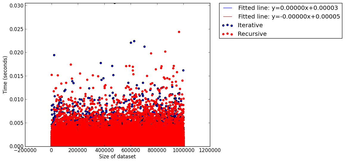
Here's a scatter plot (with fitted lines) for all the data points:

A part from the fact that binary search seems very good indeed, there's not that much going on here apart from perhaps a slight tendency for iterative approach to be a bit slower.

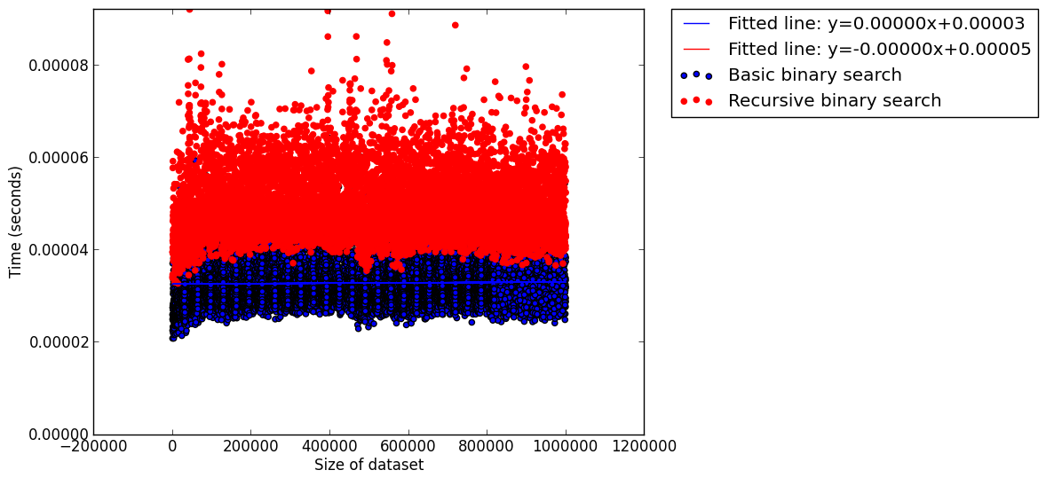
I decided to take a look at the mean time (over the 1000 searches done for each data set):

This seems to show that the iterative approach is slow but again it's not very clear. This is mainly due to the fact that I haven't done any clever analysis. The data sets are pretty big (10,001,000 data points plotted in the 1st graph and 10,001 in the 2nd) so to do anything really useful I'd have to take a look at the data a bit more carefully (the two csv files: 'recursivebinarysearch.csv' and 'iterativebinarysearch.csv' are both on github).

I thought I'd try a 'simpler' algorithm as there are perhaps a bunch of things going on with the binary search (size of data set, randomness of points chosen etc...).

Computing Factorial

The other algorithm I decided to look at was the very simple calculation of $n!$.

Iteration

Here's the simple algorithm written iteratively:

def iterativefactorial(n):
    r = 1
    i = 1
    while i <= n:
        r *= i
        i += 1
    return r

Recursion

Here's the algorithm written recursively:

def recursivefactorial(n):
    if n == 1:
        return 1
    return n * recursivefactorial(n - 1)

The experiment

This was a much easier experiment to analyse however as the timings increased I thought it would also be interesting to look at the ratio of the timings:

We see that first of all the iterative algorithm seems to perform better but as the size of $n$ increases we notice that this improvement is not as noticeable. My computer maxed out it's stack limit  so I won't be checking anything further but I wonder if the ratio would ever get bigger than 1... (This data set: 'factorial.csv' is also on github).

I'm sure that there's nothing interesting in all this from a computer scientists point of view but I found it a fun little exercise :)