Matching games in class

Last week after looking at stochastic games we looked at matching games (corresponding to Chapter 15 of my course). There's an awesome video on +YouTube describing the problem:

I thought about possibly getting 6 students to form two groups (a set of reviewers and a set of suitors); ranking each other and then getting the class to put together a stable matching. I thought twice about this though as I'm sure it's the kind of thing that could get me fired so instead I brought 3 toys along to class with me:

• A tech deck (finger skateboard: http://www.techdeck.com/)
• The best teenage mutant ninja turtle: Donatello

Both of those you can see in this picture:

• The third toy I brought was my favourite nerf gun (the 'Praxis'):

I actually named 'her' Zoe; after my wife (+Zoë Prytherch).

Three students ('A', 'S' and 'R') came down and agreed to put together their ranking of which toy they preferred:

- A: Donatello, Zoe, Deck
- S: Zoe, Donatello, Deck
- R: Donatello, Zoe, Deck

I came up with a pretty random preference for the toys:

- Donatello: R, S, A
- Deck: A, R, S
- Zoe: R, S, A


We then discussed possible matchings and allocations of the toys (if we came to a stable one A, R and S could stick with that toy for the rest of the lesson). Here is one example that's close to what was suggested (I didn't record it and I don't quite remember it):

- A gets Donatello;
- S gets Zoe;
- R gets Deck

The thing with this is that Donatello prefers R and R prefers Donatello to their current match so the above is not stable.

After some more discussion we came up with the following stable matching:

We see that whilst A is with his 'least preferred' option (the Deck): no one prefers A to their current matching so A does not have an incentive to change his current matching.

The entire matching is stable because we can't find any pair that has an incentive to move.

In class we then went over the Gale-Shapley algorithm which is an algorithm that guarantees a stable matching. A cool thing is that this algorithm gives (out of all possible stable matchings) the one that is optimal from the suitors point of view and also the worst possible one from the reviewers point of view.

In our case above the matching found is also the matching found through the Gale-Shapley algorithm so sadly for 'A' there is no stable way of matching him to anything but his worst preferred toy and 'S' gets my wife no matter what.

Playing Stochastic/Markov games in class

In class on Monday my students and I looked at Stochastic games (Chapter 14 of my course notes). I decided to play a tournament similar to the iterated games that we played previously (corresponding to Chapters 9 and 10). I've blogged about them here and here.

In short, a stochastic game is a collection of states that themselves correspond to games. After players select strategies at a given state/game the next game they play (or state they are in) is given by a probability distribution.

This is a bit like playing in a casino where the table you play at depends on what happened at the previous table you played.

*The game we played in class corresponds to a casino with two tables:*

- At the first table we play a simple prisoner's dilemma (players aiming to maximise) their utility:

$$\begin{pmatrix}
(2,2)&(0,3)\\
(3,0)&(1,1)
\end{pmatrix}$$

The probability distribution at this table (indicating what game we played next) is given by:

$$\begin{pmatrix}
(.75,.25)&(0,1)\\
(0,1)&(.5,.5)
\end{pmatrix}$$

    - If both players cooperate (getting a utility of $2$ each) then there is a 75% chance that they play at this same table again.
    - If only one player cooperates and the other defects (the defector getting a utility of $3$ and the cooperator a utility of $0$) then the players move to the other game with 100% probability.
    - If both players defect (each getting a utility of $1$) then they will play the same game with 50% chance.

- The second table was a dummy game that basically ended the game:

$$\begin{pmatrix}
(0&0)
\end{pmatrix}$$

The probability distribution for this game is $(0,1)$.

The assumption made in this class is that the games are played infinitely and as such a discounting factor $\delta$ is used. When playing this in class we interpreted the discounting factor as the probability of the game continuing. So the game ended when the probabilities indicated that we were in the second game or when the discounting factor said so (we used $\delta=1/2$).

The class formed 4 teams and we played a round robin.

The first round had Tom's Team go up against Team Roy and Barmy go up against 4:

We see that Tom's team and Team Roy cooperated both times before the game ended whilst 4 defected from the start against Barmy.

The next round had Barmy go up against Tom's Team and Team Roy go up against 4:

We see that Barmy and Team Roy both cooperated before the game ended and Team Roy and 4 both defected before the game ended.

The last game had Tom's Team go up against 4 and Team Roy go up against Barmy. Below you can also see the final cumulative scores:

As you can see Tom's Team won (the name is after +Paul Harper son Tom joined the class during which we played the iterated prisonder's dilemma).

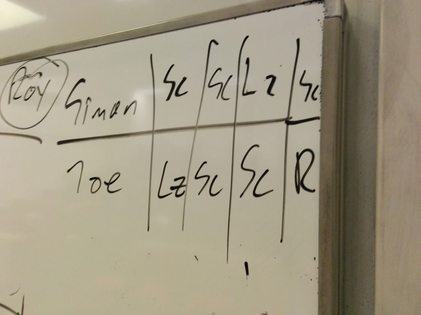
To decide who came second (they could choose the second prize to either be apples or party rings) a best of three game of Rock, Paper, Scissors, Lizard, Spock was played with Joe winning the party rings for Team Roy ('Scissors decapitates lizard').

I think this was good fun and hopefully enabled the students to have a sound grasp of what is meant by a state, a transition, etc..

Interestingly all teams happened to play Markov Strategies (i.e. in any given game they all did the same thing in each state) although this might have been different if the probabilities allowed the game to last longer. In the course we are restricting ourselves to Markov strategies.

After playing this we went through obtaining 2 equilibria for this game (both players defecting and both players cooperating).

Here are some photos that a student grabbed during the class and also a re-share of the gif of +Paul Harper's son Tom using a Nerf gun on those who defected against his team during the Prisoner's dilemma tournament:

Playing a game with incomplete information in class

In class today we took a look at games of incomplete information. Loosely this relates to any kind of game that involves the players not knowing 'everything'.

Next week we'll be looking at stochastic/Markov games (C13 of my course) but this week we took a look at incomplete information in extensive form games (C12 of my course).

We played the following game (a generalization of the matching pennies game that I've blogged about before):

"Player 1 picks Heads or Tails, a coin is flipped and Player 2 is aware of the result of that coin (but not the choice of Player 1), Player 2 then picks Heads or Tails. The is akin to a matching pennies game except that if Player 2 loses whilst picking the same as the random coin then the outcome is $(0,0)$."

Here is a game tree that describes the game:

On a slight tangent our School operates a mid-module feedback system which is not 'official' but allows us to get some feedback from students with regards to how the course is going so far. One piece of feedback I got was something like:

"The chocolates are making me fat bring fruit instead."

I'm pretty sure this was tongue in cheek but I brought in the following as a prize for the winner of a 3 player round robin (using the above game):

(A melon and some fizzy cherries)

As I said, I got 3 students (referred to as S, A. R) to play a round robin tournament where each would play each other twice (swapping being player 1).

The results are here (thanks to +Jason Young for collecting them):

In that photo we see the following match ups:

- Game 1 and Game 2: A versus S

- Game 3 and Game 4: R versus S

- Game 5 and Game 6: A versus R

What we see is that R actually won with a final cumulative score of 3, A finished with -1 and S with -2. Looking through the details we see that A and S both went "against" the coin both times whereas R went "against" the coin once.

I asked the class if anyone had an idea of how one should play the game. One student (who I think was from the team Roy crowd) yelled out that one should always go with the coin.

This is exactly correct, the way to 'prove it' it is to obtain the corresponding normal form game for the extensive form game. We do this by using expected values over the random nodes:

We have $S_1=\{H,T\}$ and $S_2=\{HH, HT, TH, TT\}$. The strategy set for player 2 indicates what player 2 should do for each possible flip of the random coin: so $HT$ indicates playing $H$ if the coin flips Heads and playing $T$ if the coin flips Tails (so $HT$ corresponds to agreeing with the coin, $TH$ corresponds to going against the coin etc...).

Using the above strategy ordering we get the following normal form game:

$$
\begin{pmatrix}
(1/2,-1/2)&(-1/2,1/2)&(0,0)&(-1,1)\\
(-1,1)&(-1/2,1/2)&(0,0)&(1/2,-1/2)
\end{pmatrix}
$$

I will skip the analysis of this game (which we did in class) but it can be shown that the Nash equilibrium is for player 1 to play Heads with probability between 1/3 and 2/3 and player 2 to agree with the random coin.

Importantly, at the end of the game the victor: R gave the melon to A. I hope he enjoys it and also that my students found this exercise slightly useful and perhaps slightly more memorable.

A (very) brief interactive look at evolutionary game theory in class

In class last week my students and I started looking at evolutionary game theory (Chapters 11 and 12 of my class). One concept of evolutionary game theory that is important to understand is that in a sense the barrier between strategies and players becomes a bit fuzzy.

To try and illustrate this in class I brought in 2 packs of cards. I actually ended up only using the cards as binary markers (whether or not they were facing 'UP' or 'DOWN'). I then proceeded to describe the following:

"If an UP card interacts with a DOWN card in any given round the DOWN card changes to UP on the next round. Otherwise everything else stays the same."

I used this game to illustrate how a strategy $\sigma$ can induce a population vector $\chi$ and I also touched upon what we would mean by $\sigma$ being stable.

We played the following games:

---------------

The left half the class was told to play UP and the other half to play DOWN. Thus our initial value of $\chi=(.5,.5)$. This was given by the fact that half the population was playing $\sigma=(1,0)$ and the other half playing $\sigma(0,1)$.

We played a couple of rounds (which was fairly academic as the outcome is obvious) and arrived at a final population vector of $\chi=(1,0)$ (all the DOWN cards had been changed to UP cards). This is a stable population.

I asked what would happen if I nudged the population by introducing some more DOWN cards in to the population, to perhaps $\chi=(.9,1)$. Everyone realised that the population would swiftly move right back to $\chi=(1,0)$.

We also talked about what would happen if we started with $\chi=(0,1)$ (all cards started as DOWN), everyone realised that $\chi$ would not change over time as we played (since there were no UP cards to force a change). This is also a stable population.

It's obvious though that if we introduce some UP cards (say nudging the population to $\chi=(.1,.9)$) then the population would swiftly move to $\chi=(1,0)$.

The difference between these two stable populations is that one stays stable under evolutionary conditions.

That basically leads us to the definition of an evolutionary stable strategy.

---------------

The next game we played was to ask students to randomly (with equal probability) assign themselves a strategy: so everyone was playing a strategy $\sigma=(.5,.5)$.

I won't go in to the details of what we did with that (mainly re-confirming the above conclusions) but the important part is to see that any given population vector $\chi$ can be induced by a strategy vector $\sigma$. This leads to the idea of considering whether or not a strategy is evolutionary stable which corresponds to whether or not it is stable in the population that it induces.

---------------

With more time I would have liked to do more with the cards and played more games...

---------------

Tomorrow we'll be talking about pairwise contest games and the connection between normal form games and evolutionary games.

Here's a video that I put together a while ago that shows some code that allows us to investigate emergent behaviour:

Iterated Prisoner's Dilemma with a twist in Class

In my last blog post I described the iterated prisoner's dilemma tournament that my students played in class: 'Iterated Prisoner's Dilemma Tournament in Class'. This was great fun and one team even got the idea of how to define a strategy in a repeated game.

That class activity corresponded to this chapter of my class during which we looked at subgame perfect Nash equilibrium.

Let us look at the Prisoner's dilemma that we played:

\[\begin{pmatrix}
(2,2)&(5,0)\\
(0,5)&(4,4)
\end{pmatrix}\]

If both players cooperate for 3 rounds then they both get a utility of \(2\times3=6\).

The next chapter of my class looks at what is called 'infinitely repeated games', in this it is assumed that players play an infinite number of rounds. We use the usual mathematical trick to handle infinite sums so that we can compute finite utilities.

For example the utility to both players for always cooperating is given by:

\[\sum_{t=1}^{\infty}\delta^{t-1}2=\frac{2}{1-\delta}\]

Where \(0 < \delta < 1\).

The utility to both players always defecting is given by:

\[\sum_{t=1}^{\infty}\delta^{t-1}4=\frac{4}{1-\delta}\]

The 'discounting factor' \(\delta\) allows us to compare these two strategies: if both players defect they do worse then if they both cooperated.

There are various interpretations for \(\delta\), one of which is the probability with which a game continues (ie we allow for the possibility for the game to end at each round), thus the above calculation become an expected value calculation.

To illustrate this I brought a dice in to class and had +Jason Young run a tournament during which the game could end based on a chosen probability.

Here are the first set of results (we played with \(\delta=.75\) so we carried on as long as my d20 < 16):

Team Laurence got pretty lucky (players are here trying to reduce the 'amount of time they spend in prison') with their roles and twice only had to play one round!

Here's the overall standings (as well as some other details):

Team Cymru's huge score can be explained by two factors: lack of luck with the dice and they also formed a coalition with team Laurence.

After this we still had 30 minutes spare in the class so I offered ending there or playing another round. My students made me smile by mostly staying and playing another round. In fact they even pointed out that technically they shouldn't be able to watch the progression of the game (ie seeing how other teams were acting). So they suggested that the teams who weren't playing would go stand in the corridor (I thought this was cool to come from them).

We also changed the value of \(\delta\) to \(.25\) (so games only continued 25% of the time). Here are the results:

This is the last round (they're on separate boards because I had to hide/erase/etc...):

The outcome was team Roy and Cymru both tied for the win at 8 (Roy did this with well timed defections and Cymru managed to cooperate successfully a couple of times).

At this point I wasn't really sure what to use as a tie breaker but someone in class yelled: 'Rock, Paper, Scissors, Lizard, Spock'. We actually played this in class a while back when we started looking at mixed strategies, I blogged about it here: 'A Rock, Paper, Scissors, Lizard, Spock Tournament in class'

Here's the outcome of that:

Joe won it for team Roy.

This was great fun and will hopefully be useful to help my students contextualise one of the ideas of this chapter: it's actually possible to find a value of \(\delta\) for which students should cooperate. I'm not sure this was made evident by the activity but we did see more cooperation for lower values of \(\delta\).

Iterated Prisoner's Dilemma Tournament in Class

On Friday my students and I played an iterated Prisoner's Dilemma tournament in class.

This is something that I've run many times before with +Paul Harper during outreach events and I've blogged about it here and +Dana Ernst ran something similar and blogged about it here (both those posts also talk about 2/3rds of the average games).

The way I do this is to split the class in to 4 teams and play a round robin of a set of 5 to 8 repetitions of the Prisoner's Dilemma:

The particular version of the game I usually use is given below:

\[
\begin{pmatrix}
(2,2)&(5,0)\\
(0,5)&(4,4)
\end{pmatrix}
\]

The utilities represent 'years in prison' and over the 3 matches that each team will play (against every other team) the goal is to reduce the total amount of time spent in prison.

This is always good fun and my final year students were no exception (more so that +Paul Harper leant me a sidekick who was allowed to use a Nerf gun when the opposite team defected - more about that here):

In this particular instance we played 8 rounds per 'duel' and it was very helpful to have +Jason Young assist me with writing down the scores etc...

Here's the overall scores which show that the team named: 'Cymru' acquired the least total score (and won a box of chocolate):

Here's all the 'duels':

The 3rd game was the most interesting (from an educators point of view).

Team 'Roy' at the very beginning of the duel stated:

'We will cooperate until you defect, once you defect we will only defect'

Both teams cooperated fully and in the final round Roy defected (whilst their opponent continued to cooperate). This all happened with no prompting from myself which is great because team Roy in effect discovered how strategies had to be defined in repeated games which must take in to account the entire history of the game.

What's also quite cool is that they described 'Tit for Tat' the strategy that won Axelrod's tournaments.

+Michael Trick pointed out that that is completely incorrect and that Roy almost described 'Tit for Tat', they in fact played what's called 'grudger' (which did not win Axelrod's tournaments).

What happened in the last two rounds of the game was also pretty interesting as some coalitions formed to try and share the box of chocolates. Some of my students showed some great game theoretical reasoning: 'we will give you all but enough chocolates for each one of us on the team'...

In class we will consider repeated games in a more rigorous setting and before playing infinitely repeated games also play a modified version of this tournament (I'll blog about that when it happens).

(Note that the name of the winning team: Cymru is Welsh for Wales and I think was partly motivated by the fact that I was wearing my French rugby shirt before the Wales France game that evening. Wales played extremely well and thrashed France.)

Best responses to mixed strategies in class

On Monday my Game Theory class and I took a look the connection between extensive form games and normal form games (leading to subgame perfection) which correspond to these two chapters of my course: C7 and C8 but before starting that we took another look at best responses to mixed strategies (this Chapter of my course).

We have been using this game quite a bit in class:

\[\begin{pmatrix}
(2,-2) & (-2,2)\\
(-1,1) & (1,-1)
\end{pmatrix}\]

We played it before and I blogged about it here. This is a slight modification of the matching pennies game where the 1st strategy corresponds to playing Heads (\(H\)) and the second to playing Tails (\(T\))

If player 1 (the row player) is playing a mixed strategy \(\sigma_1=(x, 1-x)\) then the utility to player 2 when playing player 2 plays $H$ (the first column) can be written as:

\[
u_2(\sigma_1,H)=-2x+1-x=1-3x
\]

and when player 2 plays $T$:

\[
u_2(\sigma_1,T)=2x-1+x=3x-1
\]

We can plot these two utilities here (using +Sage Mathematical Software System):

It is immediate to note that when \(x < 1/3\) player 2 should play $T$. In fact we can write down player 2's best response \(s_2^*\) to any \(\sigma_1\):

\[
s_2^*=\begin{cases}
H,&x < 1/3\\
T,&x > 1/3\\
\text{indifferent},&
\end{cases}
\]

Using all this I played the following game in class:

• I handed out sheets asking students to play against 3 separate mixed strategies \(\sigma_1\in\{(.2,.8),(.9,.1),(1/3,2/3)\}\). I will refer to these 3 rounds as R1, R2 and R3;
• Students (acting as player 2) filled in their strategies;
• I then used the following interact to sample mixed strategies according to \(\sigma_1\):

I changed the value of \(x\) as required.

Here are the three row strategies that were sampled:

• R1: TTTTTH 
• R2: HHHTHH 
• R3: TTHTTT 

This is obviously not giving the exact proportions dictated by the mixed strategy \(\sigma_1\) but that's also kind of the point. By round, here are the results.

R1

Here's a plot of the mixed strategy that was played by the entire class during round 1:

This corresponds to \(\sigma_2=(.70,.30)\), so most students seemed willing to 'trust the theory' that one should play $H$ against this mixed strategy.

4 students scored the highest score (\(7\)) and here's the strategy they all played: \(HHHHHT\), in essence they got lucky and maxed out what they could have had. If they had played the theoretical best response (to only play $H$) they would have scored: 3.

The expected value of playing the theoretical best response (always pick \(H\) against this mixed strategy is: \(6(1-3\times.2)=2.4\) (recall that \(\sigma_1=(.2,.8)\) for this round).

The mean score for this round was 1.4 and here's a distribution of the scores:

47 students who 'won' ie scored a positive score (this is a zero zum game) played \(\sigma_2=(.83,.17)\). 18 'lost' (scored a negative score) playing \(.37,.63\).

It's nice to see that there was a large amount of students who did in fact score 3.

R2

Here's a plot of the mixed strategy that was played by the entire class during round 2:

This corresponds to \(\sigma_2=(.12,.88)\), which is again pretty close to the theoretical best response.

2 students scored the highest score: 11. They once again lucked out and played the perfect response: \(TTTHTT\). If they had played the theoretical best response they would have scored 9.

The expected value of playing the theoretical best response (always pick \(T\) against this mixed strategy is: \(6(3\times.9-1)=10.2\) (recall that \(\sigma_1=(.9,.1)\) for this round).

The mean score for this round was  6.9 and here's a distribution of the scores:

60 students 'won' ie scored a positive score (this is a zero zum game) playing \(\sigma_2=(.07,.93)\). 5 'lost' (scored a negative score) playing \(.77,.23\).

R3

The third round had the students playing against a mixed strategy for which they should have been indifferent. Here's how they played:

This corresponded to \(\sigma_2=(0.62,.38)\).

There were 10 winners for this game and they scored 10 (quite a few strategy profile gave this score so I won't list them but they mainly took advantage of the fact that mostly $T$ was sampled). (The theoretical utility is in fact 0 as you can see with one of the plots above).

The mean score for this round was was .4 (which is quite close to the theoretical value of 0). Here's the distribution of the scores:

28 scored positively playing \(\sigma_2=(.64,.36)\) and 37 scored negatively playing \(\sigma_2=(.77,.23)\).

What's nice to see here is that this 3rd round is a bit more random, with an almost (stretching the definition of the word almost) equal distribution between the number of students who won and lost.

Here's a distribution of the overall scores:

The overall winner of the game (who scored the most over the 3 rounds) was Becky who played:

• R1: \(TTHHHH\)
• R2: \(TTTTTT\)
• R3: \(HHTHTH\)

For a cumulative score of: 21

This was good fun to analyse and was hopefully useful to my students to see what is meant by best responses to mixed strategies. It was particularly cool to see an 'indifferent' (again stretching the definition of the word indifferent) response to the third round.

(Like with everything for this course you can find the data, analysis scripts and everything else at this github repo)

A Rock, Paper, Scissors, Lizard, Spock Tournament in class

I just taught mixed strategy Nash equilibria to my students (http://goo.gl/evmerJ and  http://goo.gl/wMxAoY).

I thought I could use this as an excuse to play a Rock, Paper, Scissors tournament and then someone suggested I play a Rock, Paper, Scissors, Lizard, Spock tournament:

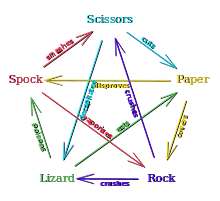
Most students had seen the game but to help us along with the rules I put this up on the board (source: wikipedia):

We then proceeded to play a 16 player knockout tournament that +Jason Young kindly helped run. Student were matched up and played best of 3 rounds with sudden death.

Here are the results (open the image in it's own tab to view it in detail):

Here's a plot of the strategies played during the 1st, 2nd and 3rd rounds:

The overall strategy profile played is here:

We're not quite playing at Nash equilibrium (which would imply a uniformly distributed choice of strategies) but it's not too far off.

Here are the strategy profiles of all matches that won a game:

Thus it looks like a response to these winning strategies would be to play strategies that beat Spock, Rock and/or Lizard. Paper would seem to be an ok bet. 

Here are the losing strategies:

It looks like Scissors was being played a bit too much and losing to Spock and Rock.

This was good fun and hopefully help the students understand what a mixed strategy is.

If it's of interest here is the dirty Python script I wrote to analyse all this.

An attempt at Golden Balls in class

Today I introduced my students to the concepts of Dominance and Best responses in my new game theory class (Chapters 3 and 4 of my class notes).

To re-affirm ideas we saw previously (normal form representation of games) and also talk about Dominance I tried to set up a kind of Golden Balls game.

Golden Balls is a game show that aired in the UK a while ago and I've never actually seen an episode but the premise is that two players cooperate during the game to come up with a total sum of money that must then be 'shared' using a Prisoner's Dilemma.

If you haven't seen this video before, it's a great example of the end game of the show:

I always show this video to students when talking about Game Theory as I reckon it's pretty awesome.

Here's what I did in class:

I got two students to play the game: A and S. They were to compete against me (as the row player, I was the column player) in the following 5 normal form games (their utility corresponded to the number of chocolates I would owe them):

1. Just a plain old matching pennies game (we played this in class last week and I blogged about it here):

$$\begin{pmatrix}
(1,-1)&(-1,1)\\
(-1,1)&(1,1)
\end{pmatrix}$$

2. A modification of this game with a weakly dominated strategy:

$$\begin{pmatrix}
(1,-1)&(-1,1)\\
(1,-1)&(1,-1)
\end{pmatrix}$$

A and S were both quick to realise  that they should play the second row strategy.

3. A modification of the matching pennies game:

$$\begin{pmatrix}
(2,-2)&(-1,1)\\
(-1,1)&(2,-2)
\end{pmatrix}$$

4. A game with a strategy at which they would definitely win something:

$$\begin{pmatrix}
(2,-2)&(1,-1)\\
(-1,1)&(2,-2)
\end{pmatrix}$$

5. The same game as 4, again (when I play this next year I'll change this game slightly).

This ended up with A and S having about 6 chocolates between them. I then split the team up and told them to play:

$$\begin{pmatrix}
(2,2)&(0,3)\\
(3,0)&(1,1)
\end{pmatrix}$$

If they cooperated (choosing the first strategy) I would double the 6 chocolates and they would have 12 chocolates each. If 1 defected, the defector would have 18 chocolates and the other none. If they both defected they would just have 6 chocolates each.

I asked if they'd like to talk to each other. S, tried but A confidently said: 'no need, I know what you are going to do'. S cooperated and A defected.

There were 1 or 2 'oooos' that were swiftly ended when A proceeded to immediately share his chocolates with A. I in fact ended up just giving the whole box of chocolates I bought:

After this we moved on to talk about best response strategies. 

I asked for a volunteer to player tic-tac-doe with me and we used this as a discussion about best responses:

'Right, now that she has played there, where should I play?'

I put up a picture of +Randall Munroe's tic-tac-toe solution.

All in all it was good fun I think and hopefully helped make the class a bit more 'alive'. I have a (what I think is a) cool idea about a game I'll try and play with my students next week when talking about mixed strategy equilibrium. This could involve a bracket of 16 volunteers...

If you liked the video above, take a look at this one which is pretty awesome too:

Matching pennies in class

Yesterday I took the first class of my new module on Game Theory. I've been very excited about this as I think Game Theory is a really fun subject to learn (and teach).

In class we covered the first two chapters of my notes (Chapter 1: Introduction to Game Theory, Chapter 2: Normal Form Games). Whilst talking about Normal Form Games I showed the students the game called Matching Pennies.

Two players each show a coin with either 'Heads' or 'Tails' showing. If both coins match then the 1st player (the row player) wins, otherwise the 2nd player (the column player) wins.

This can be represented using a 'bi-matrix':

$$\begin{pmatrix}
(1,-1)&(-1,1)\\
(-1,1)&(1,1)
\end{pmatrix}$$

Each tuple of that matrix corresponds to a pair of strategies from the set $\{H, T\}$, so if the row player chose $H$ and the column player chose $T$ then they would read the outcome in the first row and second column: $(-1,1)$. The convention used here is that outcomes show the utilities to the first and then the second player. So in this instance the row/first player would get -1 and the column/second player would get 1 (ie the column player wins because the coins where different).

I asked the students to get in to pairs and record five rounds of the game on some paper (forms and all other content for the course available at this github repo).

After that, I modified the game to give this:

$$\begin{pmatrix}
(2,-2)&(-2,2)\\
(-1,1)&(1,1)
\end{pmatrix}$$

The row player still wins when the coins match but there is just more to win/lose when $H$ is picked by the row player.

I got the students to once again record the results.

Last night I got home and instead of speaking to my wife I went through and entered all the data.

Here are some of the results.

First of all 'basic matching pennies'. Here are the moving averages of all the games played:

I'm graphing the probability with which players played $H$. As you can see 'we' got to equilibrium pretty quickly and 'on average' players were randomly swapping between $H$ and $T$.

Here is a plot of the equivalent mean score to both players:

First of all we see that the plots are reflections in the $x=0$ line of each other. This is because the game we are considering is called a Zero Sum Game: all the utility doublets sum to 0. Secondly we see that the mean score is coming around to 0. 

All of the above is great and more or less exactly what you would expect.

While playing the second game I overheard a couple of students say something like 'Oh this is a bit more complicated: we need to think'. They were completely right!

Here are the results. First of all the strategies:

It seems like students are once again playing with equal probabilities of picking $H$ or $T$. The outcome for the score is again very similar:

Is this what we expect?

Not quite.

Let us assume row players are playing a 'mixed strategy' $\sigma_1=(x,1-x)$ (ie they choose $H$ with probability $x$) and column players are playing $\sigma_2=(y,1-y)$.

Let us see what the expected utility to the row player is when $\sigma_2=(.5,.5)$ as a function of $x$ (the probability of  playing $H$):

$$u_1((x,1-x),(.5,.5))=.5(2x-(1-x))+.5(-2x+1-x)=0$$

So in fact what the row player does is irrelevant (with regards to his/her utility) as long as the column player plays $\sigma_2=(.5,.5)$.

What about the column player?

Writing down the utility to the column player when $\sigma_1=(.5,.5)$ as a function of $y$ (the probability of playing $H$):

$$u_2((.5,.5),(y,1-y))=1/2(-2y+y+2-2y+y-1)=1/2-y$$

So NOW if $\sigma_1=(.5,.5)$ it looks like the column player has SOME control over his/her utility.

Here is a plot of that $u_2$:

So our plot is that of a decreasing function. Remember $y$ is something that the column player can control. So as the column player wants to increase $u_2$: the best response they should adapt to the row player playing $\sigma_1=(.5,.5)$ is in fact $y^*=0$ because at $y=0$ the utility is at it's highest!

What this implies (for the second game) is that whilst the students were all winning and losing in equal measure (the mean score was around 0). The column player could in fact improve their strategy and take advantage of the fact that the row player was playing $\sigma_1=(.5,.5)$.

The row player can't actually do this (we did the math above and we saw that he/she couldn't really have any effect on his/her utility). What my students and I will see in Chapter 6 of my class is that in fact there is a way to make both players 'unable to improve their outcomes'. When we get there it will also shed light on the dashed lines in some of the plots of this blog post.

My Game Theory YouTube Playlist and other resources

I just added Graham Poll's awesome +YouTube playlist (http://goo.gl/UZ1Ws) to my "reading" list for my Game Theory course that I'm teaching on Monday and thought that I should also include the humble videos related to Game Theory that I have on my channel:



I also thought I could get away with making a blog post about this. The playlist above has them in 'last in first out' order but here they are in the order that I made them:

1. "An introduction to mixed strategies using Sage math's interact page."

A video that looks at the 'battle of the sexes' game and also shows of a +Sage Mathematical Software System interact.

2.  "Selfish Behaviour in Queueing Systems"

A video close to my research interests which look at the intersection of Game Theory and Queueing Theory. This video is actually voiced by +Jason Young who was doing his first research internship at the time with me and will be starting his PhD at the beginning of the 2014/2015 academic year.

3. "Pigou's Example"

A video describing a type of Game called a 'routing game'. Pigou's example is a particular game that shows the damaging effect of selfish (rational) behaviour in a congestion affected system. This video also comes with a bit of +Sage Mathematical Software System code.

4. "Calculating a Tax Fare using the Shapley Value"

This is one of my most popular videos despite the error that +Brandon Hurr pointed out at 3:51. It describes a basic aspect of Cooperative Game Theory and uses the familiar example of needing to share a taxi fare as an illustration.

5. "Using agent based modelling to identify emergent behaviour in game theory"

This video shows off some Python code that I've put online that allows the creation of a population of players/agents that play any given normal form game. There are some neat animations showing the players choosing different strategies as they go.

6. "OR in Schools - Game Theory activity"

This isn't actually a video of mine. It is on +LearnAboutOR 's channel but it's a 1hr video of one of the outreach events I do which gets kids/students using Game Theory.

7. "Selfish behaviour in a single server queue"

I built a simulation of a queue (Python code here) with a graphical representation (so you see dots going across the screen). This video simply shows what it can do but also shows how selfish behaviour can have a damaging effect in queues.

I'm going to be putting together (fingers crossed: time is short) a bunch more over the coming term.

Selfish behaviour in queues and some open source graphical simulation software

In 1969 Naor, wrote a really nice paper called 'The Regulation of Queue Size by Levying Tolls'. In this paper Naor considered a system with a single server queue:

• With an arrival rate $\lambda$ (customers per time unit)
• A service rate $\mu$ (customers per time unit)
• and a reward and cost for service that can actually just be considered as a "value for service": $\beta$

Naor then considered two types of customers: Selfish and Optimal.

It is relatively straightforward to see that Selfish customers should join if and only if:

$$\frac{n+1}{\mu}\leq \beta$$

where $n$ is the number of other customers in the system upon arrival.

What is slightly less straightforward is that Optimal customers should join if and only if $n\leq n^*$ where:

\[\frac{n^*(1-\rho)-\rho(1-\rho^{n^*})}{(1-\rho)^2}\leq \beta \mu < \frac{(n^*+1)(1-\rho)-\rho(1-\rho^{n^*+1})}{(1-\rho)^2}\]

(where $\rho=\lambda/\mu$)

It's a really cool result and one that has given rise to a lot more research (including what I mainly enjoy looking at).

I was asked recently be a colleague to give a 15 minute talk about my research to her second year OR class who will have just seen some queueing theory. I decided to talk about Naor's paper and thought that it would be nice if I could give a graphical representation of the customers arriving at the queue (similar to the DES package: +SIMUL8). So I spent some time writing a simulation engine and using the in built +Python Turtle library to get some graphics. A part from some of the optional plotting (matplotlib), this only uses base python libraries. Here's a gif from an early prototype:

Here's a video discussing Naor's result and showing demonstrating everything with my simulation model:

The code is all up on github and it really could do with some improving so it would be great if anyone wanted to contribute: https://github.com/drvinceknight/Simulating_Queues

Results from my online version of the two thirds of the average game.

In my previous blog post I described briefly the online version of the two thirds of the average game that I set up using Google's app engine (the main reason for this was to make sure I knew how to do it as I plan on using something similar in an upcoming class).

I invited people to play and kept the game going for a week. I was hoping for a few more participants than I go but it was nice to get 76 people take the time to play.

Drum roll...

The winning guess was 15 and this was guessed by a single individual who did not leave a url but whose google username makes me think their name is Dalibor Smid: so congratulations and thanks for playing :)

The distribution of the guesses is fairly traditional for this experiment with peaks at the guesses that are 2/3s of the previous peak (66,44,29, 19 etc...).

Thanks a lot to everyone for playing and also for everyone who re-shared my invitation:

• +Paul Harper 
• +Theron Hitchman 
• +Patrick Honner 
• +Matt Lowrie 
• +Zoe Prytherch 
• +John Hammersley 
• AMS Blog on Math Blogs
• @evelynjlamb
• @JulienFlaig
• @or_exchange

and others that I apologise for forgetting!

I'm going to leave the game up there and reset it. I'll let the data store fill up until reaching 200 people and then reset it again (assuming 200 poeple ever decide to play :) etc...

So if you want to have another go please do go play:

http://twothirdsoftheaveragegame.appspot.com/

Invitation to play a game

So I've blogged about the two thirds of the average game quite a few times now. The latest pos that is kind of a summary of the other posts can be found here.

This post is however a bit different. I'm teaching a new game theory course next year and am busy preparing that. I'm planning on using various interactive games to help with my teaching. As a result I've been figuring out google's app engine so that I can host some of these games online.

The result of this is that I've put together an online open version of the two thirds of the average game that I'd really appreciate you taking the time to play.

The website is: twothirdsoftheaveragegame.appspot.com/ and it will take you 3 minutes to make a guess (you're welcome to guess a bunch of times, only your last guess will count).

Thanks to +Leanne Smith, +Zoe Prytherch, +Izabela Komenda, +Penny Holborn and +Angelico Fetta for testing it for me. Hopefully the bugs are all gone :)

I'll let this run for a week and pick the winner(s) on the 3rd of May at 1200 GMT. That's a week away. I would really aprpeciate you taking the time to play and can't offer much to the winners a part from being named (if you would like me to) in my blog post I write next week :)

So please do take the take to guess, more details about the game itself can be found at the site:

twothirdsoftheaveragegame.appspot.com/

All the code for the site can be found at this github repo.