Showing posts with label LaTeX. Show all posts

Tuesday, 3 December 2013

Explaining floats in LaTeX

A PhD students recently had a hard time placing floats (figures and table environments) where they wanted in their LaTeX document. I also have just finished teaching LaTeX to all our first years here at +Cardiff University so I thought I'd brush up on my own understanding of these things to make sure that I was explaining things correctly.

I stumbled on the following stackoverflow TeX.Stackexchange (thanks to +Torbjørn Taskjelle for pointing out this and other mistakes) answer: http://goo.gl/A9iJnP

Here's a +writeLaTeX document working through some examples showing the various options that allow you to control floats within the default restrictions: https://www.writelatex.com/read/qkjpvqptqrwd (at the moment that's a read only link but I've suggested it as a template to the writeLaTeX team in case it's useful to anyone). EDIT: Here's the link to the template: http://goo.gl/UmLFr3

I think that reading through the code (which explains how I understand these things to work) could prove helpful when trying to explain how the various options work. Once that's done I'd suggest playing with the following options on the rabbit figure:

- [t]
- [!t]
- [p]
- [!h]
- [!htbp]

and others to see the effects.

If anything I've written in that document (https://www.writelatex.com/read/qkjpvqptqrwd) isn't quite right I'd appreciate being told :)

Friday, 11 October 2013

Revisiting the relationship between word counts and code word counts in LaTeX documents

In this previous post I posted some python code that would recursively search though all directories in a directory and find all .tex files. Using texcount and wc the code the script would return a scatter plot of the number of words against the number of code words with a regression line fitted.

Here's the plot from all the .tex files on my machine:


That post got quite a few views and +Robert Jacobson was kind enough to not only fix and run the script on his machine but also sent over his data. I subsequently tweaked the code slightly so that it also returns a histogram. So here's some more graphs:

  • Robert's teaching tex files:


  • Robert's research files:


It looks like my .6 ratio between code words and words isn't quite the same for Robert...

BUT if we combine all our files together we get:


So I'm still sticking to the rule of thumb for words in a LaTeX file: multiply your number of code words by .65 to get in the right ball park. (But more data would be cool so please do run the script on your files :)).

The tweaked code (including Robert's debugging) can be found in this github repo: https://github.com/drvinceknight/LaTeXFilesWordCount

Sunday, 6 October 2013

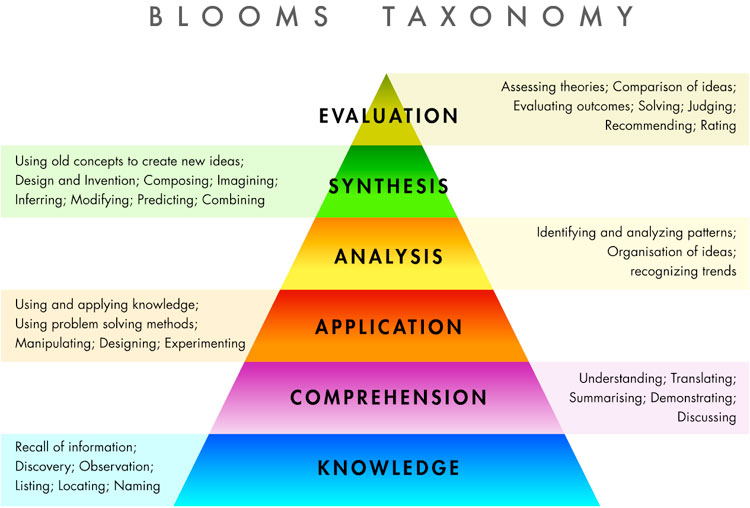
Bloom's taxonomy drawn in Tikz

I'm in the middle of writing about various pedagogic theories for PCUTL (a higher education certification process) and I needed a picture of Bloom's taxonomy:


I needed to be able to play around with it a bit (so as to add annotations and colours like in the above picture) so I wanted something in Tikz. I found this helpful stack-exchange post for hierarchical pyramids and stole modified the code from there to get Bloom's taxonomy in Tikz. Here's the stripped down version:


The code is here (I modified the following slightly to give the above standalone image using the tikz standalone document class):


\documentclass{article}

\usepackage{tikz}
\usetikzlibrary{intersections}

\title{Bloom's taxonomy}


\begin{document}
\begin{center}

\begin{tikzpicture}
\coordinate (A) at (-6,1) {};
\coordinate (B) at ( 6,1) {};
\coordinate (C) at (0,7.5) {};
\draw[name path=AC] (A) -- (C);
\draw[name path=BC] (B) -- (C);
\foreach \y/\A in {1/Knowledge,2/Comprehension,3/Application,4/Analysis,5/Synthesis,6/Evaluation} {
\path[name path=horiz] (A|-0,\y) -- (B|-0,\y);
\draw[name intersections={of=AC and horiz,by=P},
name intersections={of=BC and horiz,by=Q}] (P) -- (Q)
node[midway,above] {\A};
}
\end{tikzpicture}
\end{center}

\end{document}


I put it up on +writeLaTeX as well: here.


Saturday, 5 October 2013

Almost a 2 to 1 ratio of total code words to words in my LaTeX files...

In my previous post I posted a small python script that will recursively go through all directories in a directory and return the word count distribution using texcount (a utility that strips away LaTeX code to count words in documents). In this one I'm going to try and find a way of finding out how many words are in my LaTeX files without counting them (kind of).

On G+ +Dima Pasechnik suggested the use of wc as a proxy but wc gives the count of all words (include code words). I thought I'd see how far off wc would be. So I modified the python script from my last post so that it not only runs texcount but also wc and carries out a simple linear regression (using the stats package from scipy). The script is at the bottom of this blog post.

Here's the scatter plot and linear fit for all the LaTeX files on my system:


We see that the line $y=.68x-27.01$ can be accepted as a predictor for the number of words in a LaTeX document as a function of the total number of code words.

As in my previous post I obviously have an outlier there so here's the scatter plot and linear fit when I remove that one larger file:

The coefficient is again very similar  $y=.64x+26$.

So based on this I'd say that multiplying the number of codewords in a .tex file by .6 is going to give me a good indication of how many words I have in total.

Here's a csv file with my data, I'd love to know if other people have similar fits.

Here's the code (a +Dropbox link is here):

#!/usr/bin/env python import fnmatch import os import subprocess import argparse import pickle import csv from matplotlib import pyplot as plt from scipy import stats parser = argparse.ArgumentParser(description="A simple script to find word counts of all tex files in all subdirectories of a target directory.") parser.add_argument("directory", help="the directory you would like to search") parser.add_argument("-t", "--trim", help="trim data percentage", default=0) args = parser.parse_args() directory = args.directory p = float(args.trim) matches = [] for root, dirnames, filenames in os.walk(directory): for filename in fnmatch.filter(filenames, '*.tex'): matches.append(os.path.join(root, filename)) wordcounts = {} codewordcounts = {} fails = {} for f in matches: print "-" * 30 print f process = subprocess.Popen(['texcount', '-1', f],stdout=subprocess.PIPE) out, err = process.communicate() try: wordcounts[f] = eval(out.split()[0]) print "\t has %s words." % wordcounts[f] except: print "\t Couldn't count..." fails[f] = err process = subprocess.Popen(['wc', '-w', f],stdout=subprocess.PIPE) out, err = process.communicate() try: codewordcounts[f] = eval(out.split()[0]) print "\t has %s code words." % codewordcounts[f] except: print "\t Couldn't count..." fails[f] = err pickle.dump(wordcounts, open('latexwordcountin%s.pickle' % directory.replace("/", "-"), "w")) pickle.dump(codewordcounts, open('latexcodewordcountin%s.pickle' % directory.replace("/", "-"), "w")) x = [codewordcounts[e] for e in wordcounts] y = [wordcounts[e] for e in wordcounts] slope, intercept, r_value, p_value, std_err = stats.linregress(x,y) plt.figure() plt.scatter(x, y, color='black') plt.plot(x, [slope * i + intercept for i in x], lw=2, label='$y = %.2fx + %.2f$ ($p=%.2f$)' % (slope, intercept, p_value)) plt.xlabel("Code words") plt.ylabel("Words") plt.xlim([0, plt.xlim()[1]]) plt.ylim([0, plt.ylim()[1]]) plt.legend() plt.savefig('wordsvcodewords.png') data = zip(x,y) f = open('wordsvcodewords.csv', 'w') wrtr = csv.writer(f) for row in data: wrtr.writerow(row) f.close()

Saturday, 28 September 2013

Counting words in all my LaTeX files with Python

So today I found out about latexcount which will give a nice detailed word count for LaTeX files. It's really easy to use and apparently comes with most LaTeX distributions (it was included with my TeXlive distribution under Mac OS and Linux).

To run it is as simple as:

$ texcount file.tex

It will output a nice detailed count of words (breaking down by sections etc...). I don't pretend to be an expert in anything but I'm genuinely really surprised that I had never seen this before. I was about to write a (most probably terrible) +Python script to count words in a given file and just before starting I thought "WAIT A MINUTE: someone must have done this"...

Anyway, I've gotten to the point of not being able to watch TV without a laptop at the tip of my fingers doing some type of work so whilst keeping an eye on South Africa playing ridiculously well in their win over Australia in the rugby championship I thought I'd see if I could have a bit of fun with texcount.

Here's a very simple Python script that will recursively search through all directories in a given directory and count the words in all the LaTeX files:

#!/usr/bin/env python
import fnmatch
import os
import subprocess
import argparse
import matplotlib.pyplot as plt
import pickle

def trim(t, p=0.01):
    """Trims the largest and smallest elements of t.

    Args:
    t: sequence of numbers
    p: fraction of values to trim off each end

    Returns:
    sequence of values
    """
    t.sort()
    n = int(p * len(t))
    t = t[n:-n]
    return t

parser = argparse.ArgumentParser(description="A simple script to find word counts of all tex files in all subdirectories of a target directory.")
parser.add_argument("directory", help="the directory you would like to search")
parser.add_argument("-t", "--trim", help="trim data percentage", default=0)
args = parser.parse_args()
directory = args.directory
p = float(args.trim)

matches = []
for root, dirnames, filenames in os.walk(directory):
  for filename in fnmatch.filter(filenames, '*.tex'):
        matches.append(os.path.join(root, filename))

wordcounts = {}
fails = {}
for f in matches:
    print "-" * 30
    print f
    process = subprocess.Popen(['texcount', '-1', f],stdout=subprocess.PIPE)
    out, err = process.communicate()
    try:
        wordcounts[f] = eval(out.split()[0])
        print "\t has %s words." % wordcounts[f]
    except:
        print "\t Couldn't count..."
        fails[f] = err

pickle.dump(wordcounts, open('latexwordcountin%s.pickle' % directory.replace("/", "-"), "w"))


try:
    data = [wordcounts[e] for e in wordcounts]
    if p != 0:
        data = trim(data, p)
    plt.figure()
    plt.hist(data, bins=20)
    plt.xlabel("Words")
    plt.ylabel("Frequency")
    plt.title("Distribution of words counts in all my LaTeX documents\n ($N=%s$,mean=$%s$, max=$%s$)" % (len(data), sum(data)/len(data), max(data)))
    plt.savefig('latexwordcountin%s.svg' % directory.replace("/", "-"))
except:
    print "Graph not produced, perhaps you don't have matplotlib installed..."

(Please forgive the lack of comments throughout the code...)

Here it is in a github repo as well in case anyone cares enough to want to improve it.

Here is what calls it on my entire Dropbox folder:

$ ./searchfiles.py ~/Dropbox

This will run through my entire Dropbox and count all *tex files (it threw up errors on some of my files so I have some error handling in there). It will output a dictionary of file name - word count pairs to a pickle (so you could do whatever you want with that) file but if you have matplolib installed it should also produce the following histogram:


As you can see from there it looks like I've got some files quite a lot bigger than the others (I'm guessing latexcount will count individual chapters as well as the entire thesis.tex files that I have in there that include them...). So I've added an option to trim the data set before plotting:

$ ./searchfiles.py ~/Dropbox -t .05

This takes 5% of the data off each side of our data set and gives:


Looking at that I have a lot of very short LaTeX files (which include some standalone images I've drawn to do stuff like this). If I had time I'd see how good a negative exponential fits to that distribution as it does indeed look kind of random. I'd love to see how others' word count distribution looks...

Now, I can say that if I ever produce more than 600 words then I'm doing above average work...

Sunday, 15 September 2013

A playlist of short intro to LaTeX videos using the cloud based writeLaTeX.com

I've just finished screencasting, editing and uploading 21 videos to a playlist on +YouTube.

Quite frankly I'm exhausted (I started this morning), it's been a long day and I'll be happy to not have to drag another 'Ken Burns' effect boundary box around for quite a while...

Anyway, the videos are for a new course I'm teaching our +Cardiff University first year undergraduates. LaTeX has never actually been on the curriculum before and I'm throwing it in at the end of a long term (where students will mostly be learning Python and +Sage Mathematical Software System).

There are a bunch of really really great LaTeX tutorials all over the web but I thought I'd put together really short videos (the longest is around the 4 minute mark but all the others are less than 2 minutes) that just show syntax. By watching these videos no one will be a LaTeX expert (that's where the other tutorials come in).

The other particularity of these videos is that I've done them entirely using +writeLaTeX (https://www.writelatex.com/) which is a great cloud based LaTeX environment. If you don't know about writeLaTeX take a look at this great video by +John Hammersley (1 of the guys behind +writeLaTeX):


The great advantage of writeLaTeX is that I can include 2 links in the description of every video I've put together:

1. A link that creates a blank document so that anyone watching my video can right then and there try out the code.
2. A 'read only' link to the actual document I used during the video. Once this document is being viewed anyone can choose to make a copy of it so that they can play with the actual finished article.

For example: here's the video showing how to include inline mathematics:


1. Here's the link to a blank document.
2. Here's the link to the code created in the video. On the top right of that document you should see this link (which allows you to create your own copy that you can edit):


I'm hoping this will all be quite helpful to my students and in particular encourage the use of LaTeX by removing certain difficulties that some have with the installation process.

I'm also making these videos public in case they might be helpful to others (a large chunk of the videos I've put together for the programming aspects of this course are 'Unlisted' as I don't think they'd interest anyone).

Anyway the whole playlist can be found here.

There are a couple of other cloud based LaTeX environments out there (sorry for mentioning them here +John Hammersley!) including the 1 that is a part of the ridiculously awesome https://cloud.sagemath.com/. At the moment though, the user friendliness and amazing response to users (on G+ +writeLaTeX are extremely helpful) makes this an ideal tool for learning LaTeX.

Sunday, 16 June 2013

Why and how: open education resources.

This is the fourth post in a series of posts reflecting on the teaching and learning in a recent course I've taught on SAS and R. This post will be quite different in nature to the previous posts which looked at students choices between SAS and/or R in their assessment:
Here I would like to talk about how I deliver teaching materials (notes, exercises, videos etc) to my students.

All of the teaching materials for the course can be found here: drvinceknight.github.io/MAT013/.

How they got there and why I think it's a great place for them to be will be what I hope to discuss...

A Virtual Learning Environment that was not as good as alternatives.

At +Cardiff University we have a VLE provided that is automatically available to all our students that all lecturers are encouraged to use. So when I started teaching I diligently started using the service but it had various aspects that did not fit well with my workflow (having to upload files on every change, clunky interface that actually seemed optimised for IE and various other things). It was also awkward (at the time, I believe that this has been addressed now) for students to use the environment on smart phones etc...

As an alternative, I setup a very simple website using google sites and would use +Dropbox's public links to link pdfs and other resources for my students. An example of such a delivery is these basic Game Theoretical materials. This gave me great control, I no longer had to mess around with uploading versions of files, every change I made was immediately online and also as the site was pretty simple (links and pdfs) it was easily accessible to students on all platforms (I could also include some YouTube videos).

An immediate consequence of this approach is that my materials are all publicly available online.

To anyone, our students or not. The first thing I did was check with +Paul Harper: the director of the MSc course that I was only teaching on at the time that this was ok. We chatted about it a bit and were both happy to carry on. My main train of thought was that there are far better resources already available online so mine might as well be. (I've subsequently checked with our School's director of learning and teaching and there's no internal regulations against it which is nice to know about +Cardiff University)

There is a huge amount of talk about open access in research (I won't go in to that here) but less so to some extent in teaching. I did find this interesting newspaper article that ponders as to "Why don't more academics use open educational resources?". This offers a good general discussion about open education resources.

I would feel very very humbled if anyone chose to actually use my resources. I'm at the early part of my career and am still learning so I don't think that will happen anytime soon but there is another more important benefit to having my teaching stuff online for everyone.

I always post about any new courses I'm working on, on G+ and am grateful to get a fair bit of feedback from other academics around the world. This in itself gives me a certain level of confidence in front of my students who know that what I'm teaching them is verifiable by anyone in the world. I've often changed a couple of things based on feedback by other academics and I think that's brilliant.

To some extent my teaching resources are not just reviewed by a couple of peers in my university but also by anyone online who might be interested in them.

(It would be great if research worked this way too)

Through G+ (I've posted about how awesome a tool G+ is as an academic personal development tool) I learnt about git and github. If you don't know about git watch this video by +Zoë Blade is very helpful:


After a while I jumped in and starting using it. After a little longer while I found out that you can use github to host a website:


Using this I it is really easy to put together a very basic website that has all the teaching materials. The added benefit is that the materials are now all in a github repo which opens them up even more (using dbox, only the pdf files were in general in view) whereas now everything is (md, tex source files etc...) and theoretically if anyone wanted to they could pull etc...

I'm certainly not the first person to put teaching stuff up on github, (watching people like +Dana Ernst+Theron Hitchman and various others do it is what made me jump in).

The github repo for my R and SAS course can be found here and here are some other teaching things I have up on github (with the corresponding webpage if I've gotten around to setting it up):
To finish off here are the various reasons I have for putting my teaching stuff up on github:
  • Openness:
    • my students know that this is viewable by everyone which hopefully gives the resources a level of confidence;
    • people on G+ and elsewhere are able to point out improvements and fixes (if and when they have time);
  • Access: the sites are really simple (basic html with links) so they can be viewed on more or less anything;
  • Ease of use: I don't have to struggle to use whatever system is being used. If it's an option I kind of refuse to use stuff that makes me less efficient (an example of this is our email system: I use gmail). At the moment the system I like is github + git.
I wrote a blog post (which is the most read thing I've ever written - online or offline - I think) showing how to combine various things like tikz, makefiles, +Sage Mathematical Software System etc to automate the process of creating a course site so I'll put a link to that here.

Monday, 8 April 2013

Using sed to make sure hyper links refer to the correct format of file when using pandoc

In a previous post (which is by far the most popular thing on this blog which is mainly due I believe to a kind retweet by +John Cook and SciPyTip) I describe the makefiles I use to write large documents containing Tikz diagrams and +Sage Mathematical Software System plots in multiple formats (pdf, html and docx) using markdown and pandoc.

This is a short follow up post to fix one minor thing. In the previous post if you created hyper links in your markdown file (say pointing to another markdown document, which for my purposes was multiple chapters in some teaching notes) then all the formats (pdf, html and docx) would all point to the same format.

Here's a slight modification of the pandocipy_given_file.py script (from the previous post) which will use sed to replace the .md to the relevant format in all links.

#!/usr/bin/env python
from sys import argv
from os import system

e = argv[1][:-3]
print e

system("sed 's/.md/.html/g' %s > tmp" % (e + ".md"))
system("pandoc -s tmp -N -o " + e + ".html --mathjax")
system("sed 's/.md/.docx/g' %s > tmp" % (e + ".md"))
system("pandoc tmp -o " + e + ".docx")
system("sed 's/.md/.pdf/g' %s > tmp" % (e + ".md"))
system("pandoc tmp -N -o " + e + ".pdf --latex-engine=xelatex")
system("rm tmp")

This script creates a temporary file (tmp- this is actually important to make sure that the makefile doesn't think that you're recurrently changing the md files) that sed makes sure has the correct format for each link and pandoc can use to get the required files. For example the sed 's/.md/.html/g' command will replace all instances of ".md" with ".html". If you're not familiar with sed it's a *nix program that allows you to do find and replace in files "easily" (it's still a bit of voodoo to me). The script can be used by simply typing:

python pandocipy_given_file.py file.md

(Which assumes that file.md has all links sending to other md files.)

I use this script in the makefile as I did in the previous post:

md = $(wildcard *.md)
htmls = $(md:%.md=%.html)

all: $(htmls)

%.html: %.md
    ./pandocipy_given_file.py $<
    ../Scripts/generate_website.py

The final line of that file is not relevant to this blog post but it just runs a python script that will generate the website for the course (which is still a work in progress!). That python script doesn't do anything fancy but it goes in to each Chapter document for example and reads the Chapter title which it uses to write the index.html file. All this allows me to modify a given md file and simply run make to update the website file.

If any of this is of interest the github repo is here.

Note that in this particular case the links being "format loyal" is mainly useful for the `html` files to the general audience. The loyal links in pdf and docx format are mainly useful to me as all the paths are relative to my setup. I'm posting this again so that I don't forget it but also in case it's useful to others (you can obviously use sed to replace other things).

Sunday, 7 April 2013

Makefiles for tikz sagemath and teaching notes written in markdown

So I've posted before on multiple occasions about PCUTL which is a higher education certification process I'm currently undergoing. One of the things I paid particular attention to in my latest portfolio (a copy of which can be found at the previous link) is accessibility of teaching notes.

Generally this implies making sure students have notes in a format that they can easily manipulate (for example change font size and color). This is often implied to mean that notes should be written in .doc format. As a mathematician this isn't really an option as all our teaching material really requires to be written in LaTeX.

I have spent some time being amazed by pandoc which is a really smart piece of software that allows you to take documents in various languages and output to a variety of other languages. Here's a video I made showing how I use like to use pandoc to get notes in html,pdf and .docx format (I wrote a blog post here about it):


My entire SAS/R programming course I'm currently teaching was written this way (you can find the notes etc here).

I've recently started writing a new course: a game theory course.

This course needs a bunch of diagrams and plots (as opposed to the previous that basically had a bunch of screenshots). I wanted to use the same overall system but planned on using tikz for the diagrams (tikz lets you draw nice diagrams using code) and perhaps thought about using sagetex (I use +Sage Mathematical Software System a lot but have never used sagetex which lets you have sage code inside of a LaTeX document) for the plots.
After searching around for a bit I didn't see how I was going to be able to use the awesome pandoc to create teaching notes in multiple formats using the above approach. There was no way for pandoc to take the tikz code and output a separate image file for the html (and whatever it needs for .docx).

This blog post is a summary of my approach.

Which basically uses a couple of things:
  • Some tikz code that creates a standalone pdf image;
  • A script that converts a pdf to a png (so that it can be used in html);
  • A makefile so that I can recompile only the tikz code that needs to be recompiled;
That is how I get my tikz diagrams.

I also have a similar system to create plots from sage and I'll also show the makefile I use to get pandoc to sort out the files I want.

Creating standalone pngs with tikz and makefiles


To create a standalone tikz image you need to use the standalone document class. Once you've done that you can just use normal tikz code:

\documentclass[tikz]{standalone}
\usepackage{tikz,amsmath}
\tikzstyle{end} = [circle, minimum width=3pt, fill, inner sep=0pt, right]
\begin{document}
\begin{tikzpicture}
    \draw (0,0) -- (4,0) node [below] {$u_1$};
    \draw (0,0) -- (0,4) node [left] {$u_2$};
    \draw (3,0) node[end] (A) {} node [above=.3cm,right] {$(3,0)$};
    \draw (0,3) node[end] (B) {} node [above=.3cm,right] {$(0,3)$};
    \draw (1,1) node[end] (C) {} node [below,left] {$(1,1)$};
    \draw (2,2) node[end] (D) {} node [above=.3cm,right] {$(2,2)$};
    \draw (A) -- (D);
    \draw (D) -- (B);
    \draw (B) -- (C);
    \draw (C) -- (A);
    \draw [dashed,thick] (C) -- ++(0,1.5);
    \draw [dashed,thick] (C) -- ++(1.5,0);
    \draw [->] (2,3.5) node[above] {\tiny{Feasible average payoffs}} -- (.75,2);
    \draw [->] (4,1.5) node[above] {\tiny{Individually rational payoffs}} -- (1.5,1.25);
\end{tikzpicture}
\end{document}

The above for example creates the following standalone image (note that if you pdflatex it you obviously get a pdf which would be great if you were just pdflatex'ing a bigger document but I'll get to creating a png next):


I've then written a short python script (I'm sure this could be done as easily in bash but I'm just more comfortable in python) that can act on any given tex file to convert it to png:

#!/usr/bin/env python
from sys import argv
from os import system

system("pdflatex %s" % (argv[1]))
system("convert -density 300 %s.pdf %s.png" % (argv[1][:-4], argv[1][:-4]))

This makes use of convert which is a program that can convert pdf to png (more info here but it's natively on Mac OS and *nix I believe).

I call that python file convert_tex_to_png.py and so I can convert any tex file by doing:

python convert_tex_to_png.py file.tex

I'm going to put all these image files (tex and png) in a folder called images and there's (now that I'm done) about 70 image files in there so every time I change or write a new tex file I don't want to compile all the files and I also don't want to have to waste time compiling the particular file I've written.

So I've used makefiles.

Now I've tried to use makefiles before but in all honesty they confuse the heck out of me. I spent a while going through a bunch of tutorials but most of them look at c code. For those who don't know, a makefile is basically a short program that gives instructions to compile certain files. When written well these are great as by simply typing make you can recompile any file that has been modified (and not necessarily all of them!).

So here's the makefile I've converged to using (after heuristically trying a bunch of stuff from stackoverflow):

tex  = $(wildcard *.tex)
pngs = $(tex:%.tex=%.png)

all: $(pngs)

%.png: %.tex
    ./convert_tex_to_png.py $<;

clean:
    rm *.aux
    rm *.log
    rm *.pdf

I save the above file calling it `makefile` so that it is run by default when calling `make`. This will take all the tex files (that have been modified) and output the corresponding png files as required. Note I can also type make clean to remove all auxiliary files (aux, log and pdf).

I find this really useful as I can modify a bunch of tex files and once I'm ready simply run make to get all the pngs as required.

I'll briefly show the (basically same) code I use to get plots from sage as standalone pictures.

Creating standalone pngs with sage and makefiles


I put all the plots created via sage in a plots directory. Here's an example graph created with sage:


The sage code to do that is here:

f(a,b)=a^3/3+3/4*b^2+(1-a-b)^2/2
p = contour_plot(f,(0,.5),(0,.5),colorbar=True,axes_labels=["$\\alpha$","$\\beta$"],contours=100, cmap='coolwarm',fill=True)
p.axes_labels(['$\\alpha$','$\\beta$'])
p.save("L18-plot01.png")

The makefile (which will keep all png files up to date based on the sage files in the directory):

sage  = $(wildcard *.sage)
pngs = $(sage:%.sage=%.png)

all: $(pngs)

%.png: %.sage
    sage $<;

clean:
    rm *.py

(I can similarly use make clean to remove the .py files that get created when running sage in cli).

The final thing I'll show is how to write a makefile to get pandoc to output the required file formats.

Using a makefile with pandoc


So I write all of my notes in markdown. For various reasons which include:
  • Pandoc likes markdown as input (it can also handle tex and html though);
  • I like markdown;
  • I can incorporate latex in markdown when needed.
  • If a student ever wanted to modify the markdown but didn't know LaTeX they'd have an honest chance of knowing what was going on (if you don't know markdown it really is worth taking a look at this short video)
Thus my makefile must be able to compile all modified markdown files. I use a similar approach to the approach I had for tikz diagrams which is to write a short python script:

#!/usr/bin/env python
from sys import argv
from os import system

e = argv[1][:-3]
print e

system("pandoc -s " + e + ".md -N -o " + e + ".html --mathjax")
system("pandoc " + e + ".md -o " + e + ".docx")
system("pandoc " + e + ".md -N -o " + e + ".pdf --latex-engine=xelatex")

(pandocipy_given_file.py is the name of the above python script).

There are basically three pandoc commands going on there. The first creates the html with the LaTeX math being rendered by mathjax, the second creates the .docx format and the last one creates the pdf (using the xelatex engine).

The final piece of the puzzle is to use the following makefile:

md = $(wildcard *.md)
htmls = $(md:%.md=%.html)

all: $(htmls)

%.html: %.md
    ./pandocipy_given_file.py $<;

The way that makefiles work (I think) is to indicate what files you want as an output (and what those files are dependent on). So for example my previous makefiles wanted to output pngs with tex and sage files as dependencies. Here I use the required output as html and the dependencies are the md files.

Using the above I can change any md file and simple type make to get all the pdf, html and docx files updated.

Summary and a couple of things I don't want to forget


I have 3 directories here. The first: Course_notes contains the md files and corresponding python script and makefile. Course_notes also contains 2 other directories: images and plots which both contain the images and plots as I've described above.

So in the md files I refer to an image as so:

![A pic for C1](images/C01-img03.png)


I'm using pdf as the prescribed format of the notes for the course (students are welcome to use html and docx if they wish but I'm recommending pdf) and in general xelatex will sometime move images around to better format the text.

To make sure things don't get confusing I want to be able to \ref and \label images. The easiest way I've found to do this without messing around with the html (who knows what happens with docx, life is too short to worry about everything) is to use the \text:

In the excellently drawn image shown\text{ in Figure \ref{C01-img03}} we see that...

![A pic for C1\label{C01-img03}](images/C01-img03.png)

Pandoc is clever enough to simply ignore what is in the \text when converting to html and docx so that you get documents in html and docx that won't have a reference to the figure (but in general they won't reorder the images) and the pdf will have the documents referenced as you can see in these screenshots (showing pdf and html):

pdf:

html:


I've mainly posted this to make sure I remember how to do it but it might be helpful for others. I'm sure it could be improved by getting rid of my python scripts and having everything in the makefile. I tried that but had a hard time getting wildcards to work as I did so I didn't try anything more complicated. Finally there are ways to get makefiles to run makefiles in subdirectories so it would be nice I guess to also do that so that a single `make` in the highest directory would sort out everything.

I'll be putting all the teaching notes up on github so will link to that repository when I've done it.

EDIT: Here's the github repo and here's a website with all the content (which will eventually become the class website).

ANOTHER EDIT: Here's a follow up post which uses sed to keep the links in the right format.